Eastern Bering Sea survey and fishery maps

Show/hide R code

knitr::opts_chunk$set(collapse = FALSE, comment = "#>", fig.width = 7, fig.height = 5)
library(AKsf)
library(ggplot2)

AKsf supplies a common coastline and Alaska Albers coordinate system for maps of pollock surveys and seasonal catch. This article brings together nine maps from the pollock mapping project: bottom-trawl CPUE and temperature, AVO and acoustic-trawl survey (ATS) comparisons, shaded log values, and seasonal catch with bathymetry.

Snapshot: 30 September 2026. These saved figures use the supplied inputs; the 2026 B-season catch extract ends on 18 September 2026. The figures are included unchanged for offline viewing. The runnable example below uses synthetic observations. Original survey records and fishery haul extracts are held separately from the package. The figure manifest records SHA-256 checksums for the nine included images.

A small, runnable AKsf example

Put one record on each row, retain its year and units, then turn longitude and latitude into spatial points. This example needs only the installed package and its dependencies; it downloads no data and needs no GMT installation. Point size represents catch in tonnes, rather than a density per unit area.

Show/hide R code

# Invented values for illustrating the data structure and plotting steps.
example_catch <- data.frame(
  year = rep(2026L, 6),
  season = c("A", "A", "A", "B", "B", "B"),
  lon = c(-176.5, -174.3, -170.7, -168.3, -165.4, -162.9),
  lat = c(59.5, 58.8, 57.8, 57.1, 56.1, 55.5),
  catch_t = c(250, 700, 400, 950, 600, 300)
)
stopifnot(sum(example_catch$catch_t) == 3200)

catch_points <- sf::st_as_sf(
  example_catch, coords = c("lon", "lat"), crs = 4326, remove = FALSE
)
catch_points <- sf::st_transform(catch_points, proj_aksf())

ggplot() +
  plot_coast(fill = "grey85", colour = "grey60", linewidth = 0.15) +
  geom_sf(data = catch_points, aes(size = catch_t), colour = "#a34ec4") +
  scale_size_area(max_size = 7, name = "Catch (t)") +
  coord_aksf(
    default_crs = sf::st_crs(4326),
    xlim = c(-178.8, -158), ylim = c(54, 62.3), expand = FALSE
  ) +
  theme_aksf() +
  labs(title = "Synthetic catch example", caption = "Invented observations; AKsf coastline")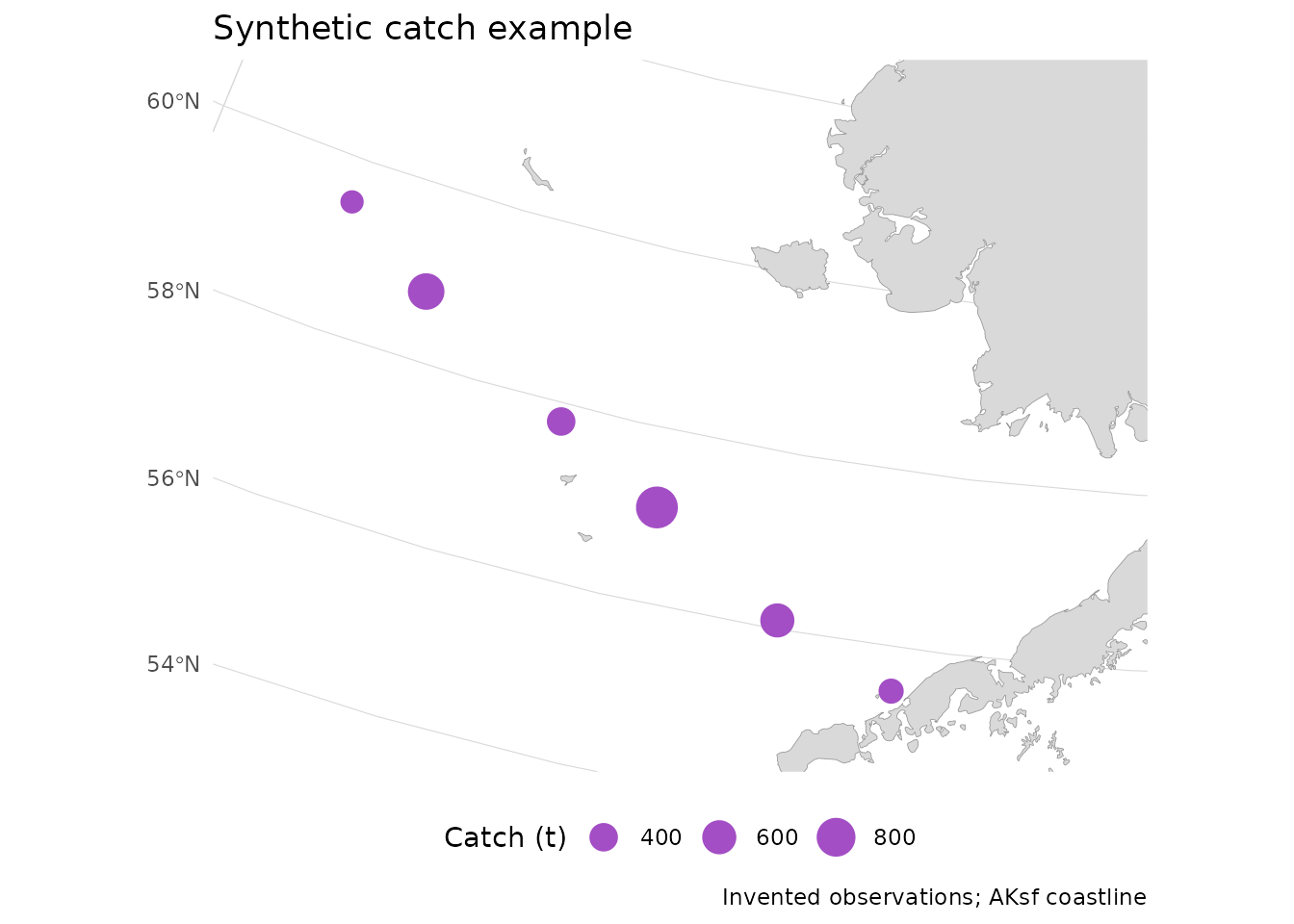

For GMT, export the same bundled coastline with write_gmt(). This writes a WGS84 GMT/OGR polygon file, preserving polygon parts and holes. The exported coordinates are longitude and latitude; distances in the R workflow use proj_aksf() (EPSG:3338, metres).

Show/hide R code

coast_file <- tempfile(fileext = ".gmt")
write_gmt(get_coast(), coast_file)
stopifnot(file.exists(coast_file), file.info(coast_file)$size > 0)
unlink(coast_file)

See Use AKsf boundaries in GMT for the GMT 6 map commands and grid handling. AKsf provides the geometry and export interface. The survey gridding, paired perspectives, and terrain rendering below belong to the application workflow.

Survey distributions

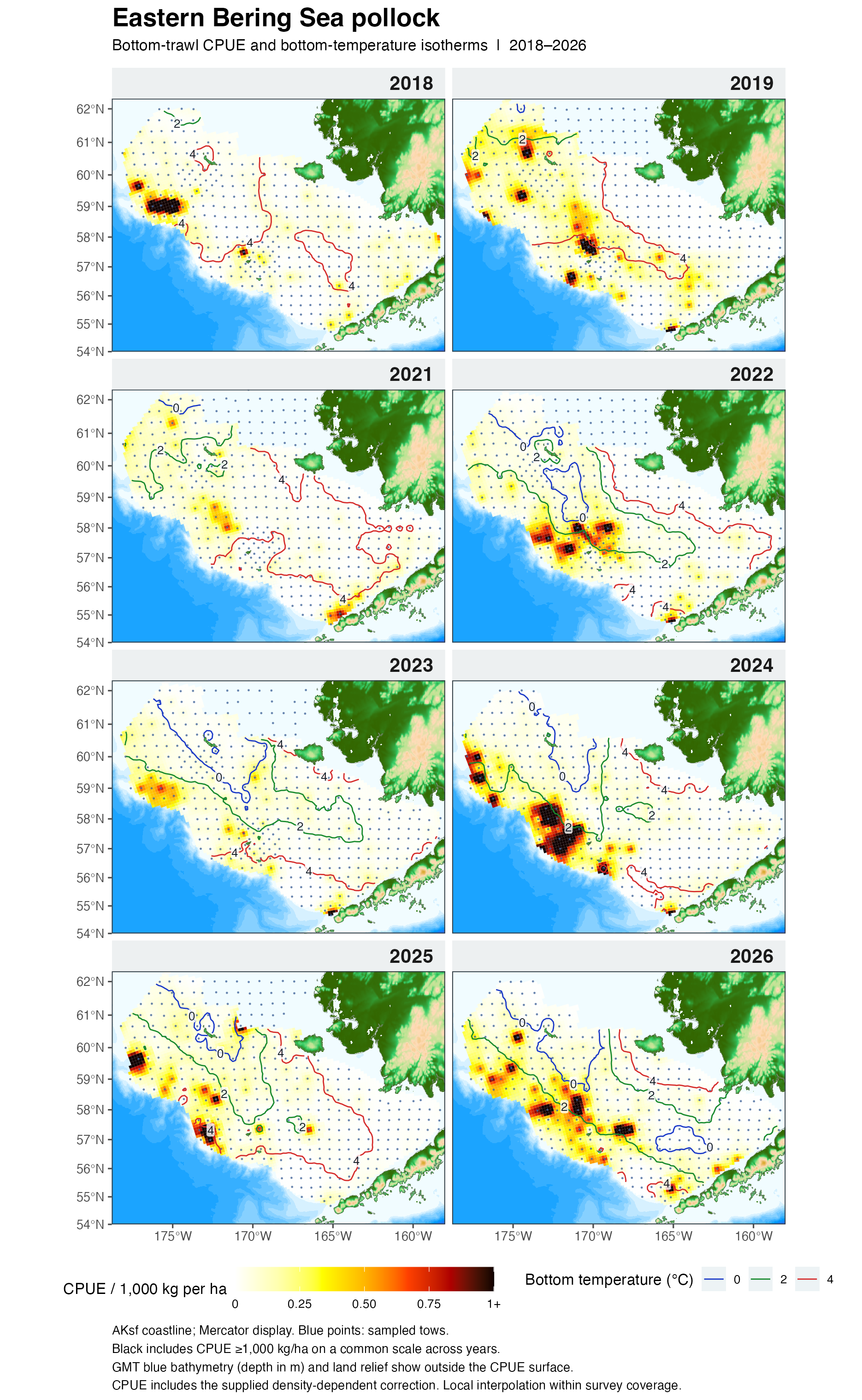
The annual bottom-trawl panels show 2018, 2019, and 2021–2026. The supplied series has no 2020 panel. CPUE uses the supplied density-dependent-corrected ddc_cpue_kg_ha values; the correction version and final adoption status are unspecified in the source CSV. Bottom temperature is in degrees Celsius. Missing temperature readings are excluded from that layer while eligible CPUE observations remain available.

Annual eastern Bering Sea bottom-trawl pollock CPUE maps for 2018, 2019, and 2021 through 2026. White to yellow, red, and black indicate increasing CPUE on a shared scale capped at 1,000 kilograms per hectare. Blue, green, and red lines show 0, 2, and 4 degree Celsius bottom-temperature contours.

Open full-size figure

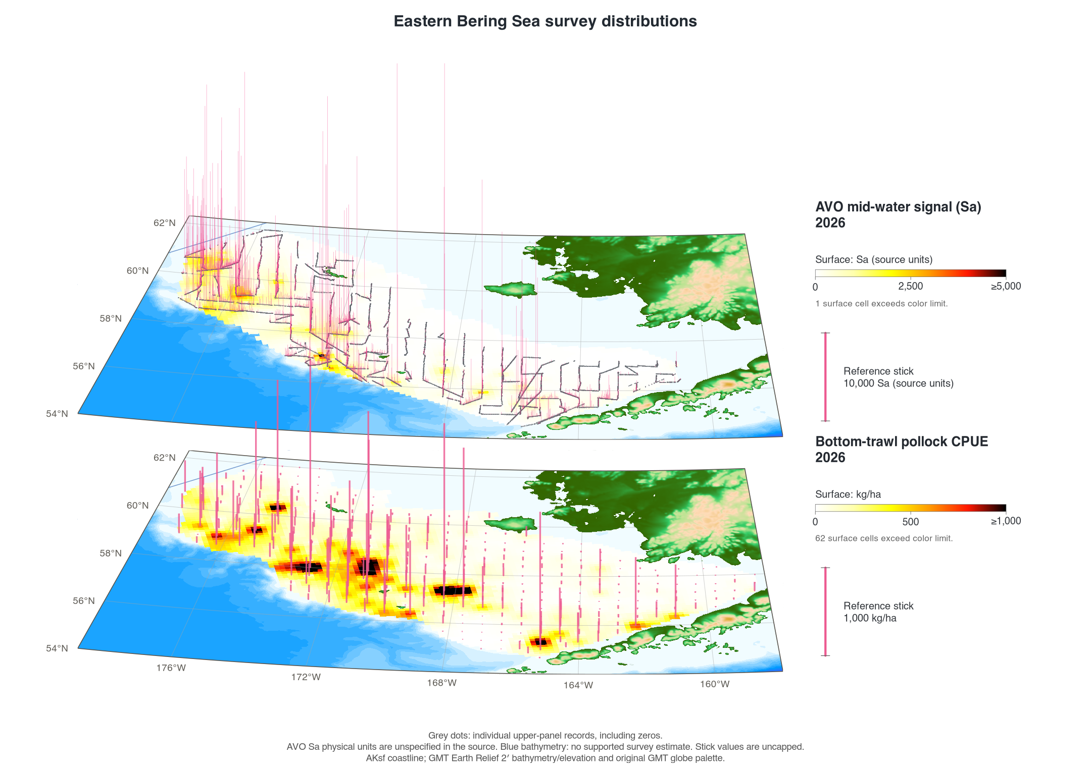
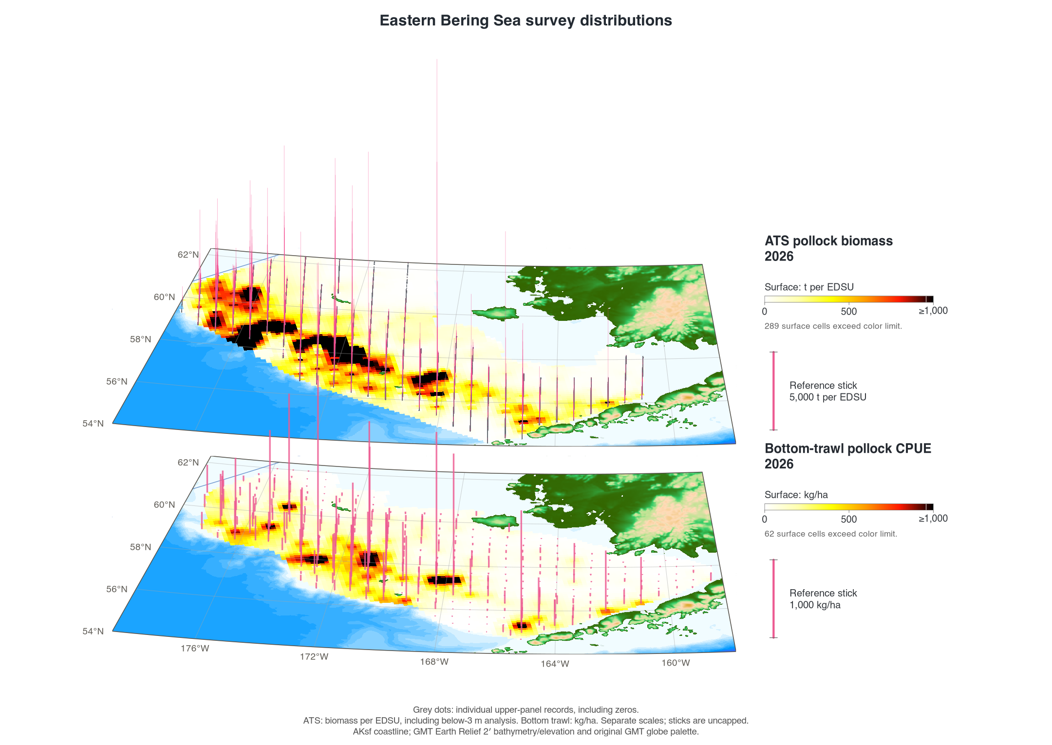
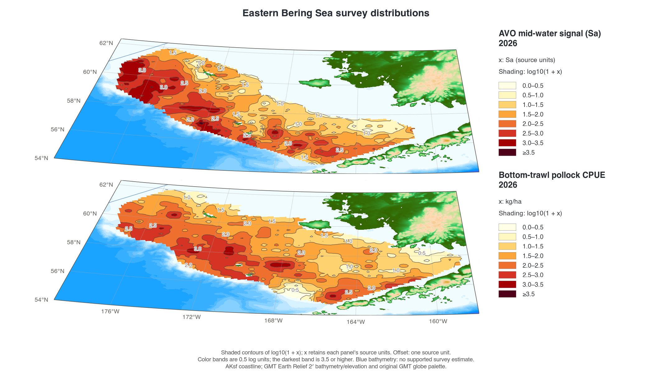
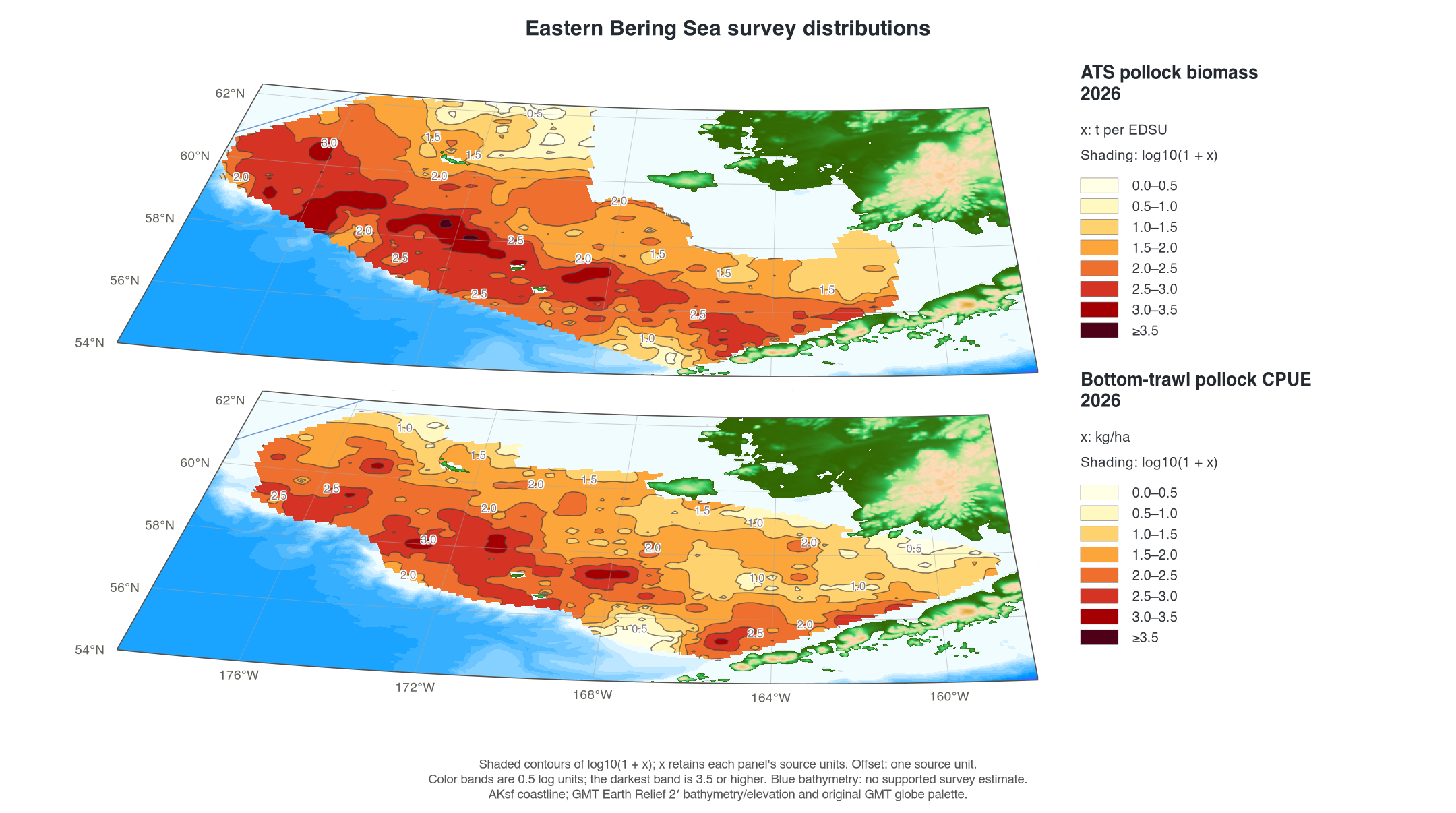
The paired views place the two map planes close together with the same camera and spatial alignment. Grey points mark each AVO or ATS record in the displayed region, making the transects visible. Pink sticks retain uncapped observed values; surface colors have their own limits.

AVO above bottom trawl, 2026

The 2026 AVO results are preliminary. AVO values are Sa in the source units; their physical units are unspecified in the input headers. The bottom-trawl panel remains kg/ha. The panels have separate scales.

Two aligned eastern Bering Sea map planes for 2026. AVO Sa is shown above bottom-trawl CPUE, with grey upper-panel record points tracing the transects, pink uncapped sticks, and white-to-black interpolated surfaces over colored bathymetry.

Open full-size figure

ATS above bottom trawl, 2026

ATS uses the supplied biomass_ton tonnes assigned to each elementary distance sampling unit (EDSU), including the source’s below-3 m analysis. The source has no EDSU-area denominator for conversion to kg/ha. All listed contributions are positive; unlisted intervals have unknown values. These biomass contributions and bottom-trawl CPUE retain their separate units.

Two aligned 2026 eastern Bering Sea map planes. ATS biomass contributions in tonnes per EDSU appear above bottom-trawl CPUE in kilograms per hectare. Grey points trace the supplied ATS records; both surfaces and pink sticks retain separate scales.

Open full-size figure

Shaded log values

These views transform the existing interpolated values using log10(1 + x) before color-limit clipping. Here x retains each panel’s source units. Missing cells remain missing. Shading uses 0.5-log-unit bands; the darkest band starts at 3.5. A log value of 1, 2, or 3 corresponds to 9, 99, or 999 in the original units. ATS remains a biomass contribution per interval, rather than an area-based density.

AVO above bottom-trawl CPUE in 2026, with colored contour bands of log10 of one plus the interpolated source values. The two planes retain their source-specific units.

Open full-size figure

ATS above bottom-trawl CPUE in 2026, with colored contour bands of log10 of one plus biomass per EDSU or CPUE, respectively. Unsupported survey cells reveal the blue bathymetry.

Open full-size figure

How the survey surfaces were made

Records were averaged in 0.3° longitude by 0.15° latitude blocks, then gridded at 10 km in EPSG:3338. Weights are proportional to 1 / distance²; up to eight blocks within 65 km contribute to a cell. Cells outside the observed convex hull, search radius, map region, or ocean remain missing. Bottom-trawl CPUE and temperature also use the archived survey polygon; AVO and ATS use their own spatial support.

These are descriptive interpolations, with no estimated spatial prediction uncertainty. They differ from the historical GMT nearneighbor and surface calculations. Review the survey mask when coverage changes. Two-dimensional annual panels use a Mercator display; paired survey views use a perspective of the common projected coordinates.

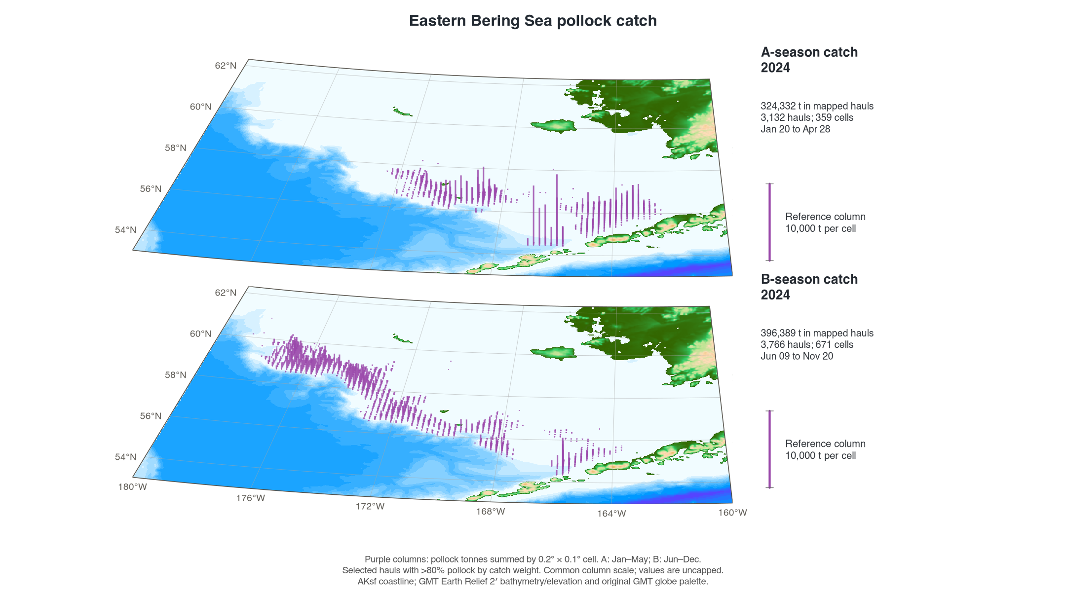
Seasonal fishery catch

A season is January–May and B season is June–December. The maps select hauls in NMFS areas satisfying 500 < nmfs_area < 540, with more than 80% pollock by catch weight, across all source vessel types. Pollock kilograms are converted to tonnes and summed in 0.2° longitude by 0.1° latitude cells. Columns represent those selected source-haul totals, with no interpolation or expansion to fleet catch-accounting totals.

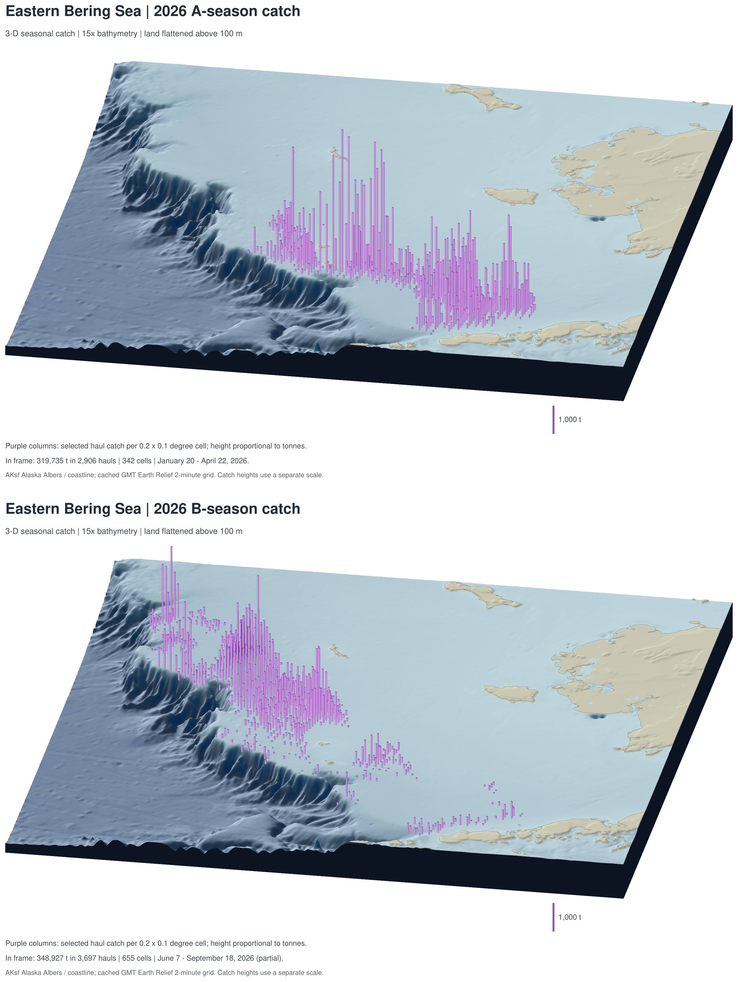
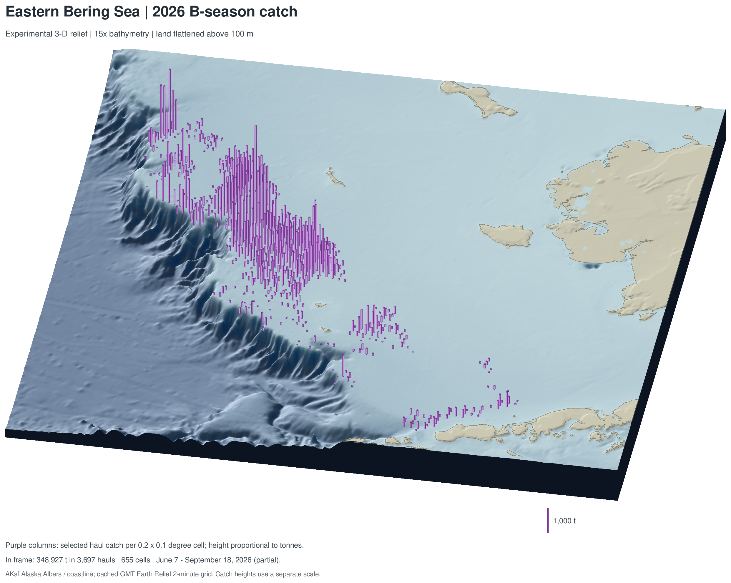
2026: three-dimensional terrain

Both seasons share the expanded, west-shifted frame, 25° viewing elevation, 170° azimuth, 15× terrain exaggeration, and a 1,000-tonne reference column. Land above 100 m is displayed at 100 m. Purple columns have a constant footprint, heights proportional to tonnes, and bases on the displayed terrain. Their heights represent catch, rather than measured tow depth.

Within the frame, A season shows 342 cells, 2,906 hauls, and 319,734.9 t (20 January–22 April); B season shows 655 cells, 3,697 hauls, and 348,927.1 t (7 June–18 September). The 2026 B season is partial.

Aligned 2026 A- and B-season catch maps, with A above B, on shaded three-dimensional eastern Bering Sea terrain. Purple catch columns share a 1,000-tonne reference. Bathymetry has 15-fold exaggeration, land is capped at 100 metres, and the B-season extract is partial through 18 September.

Open full-size figure

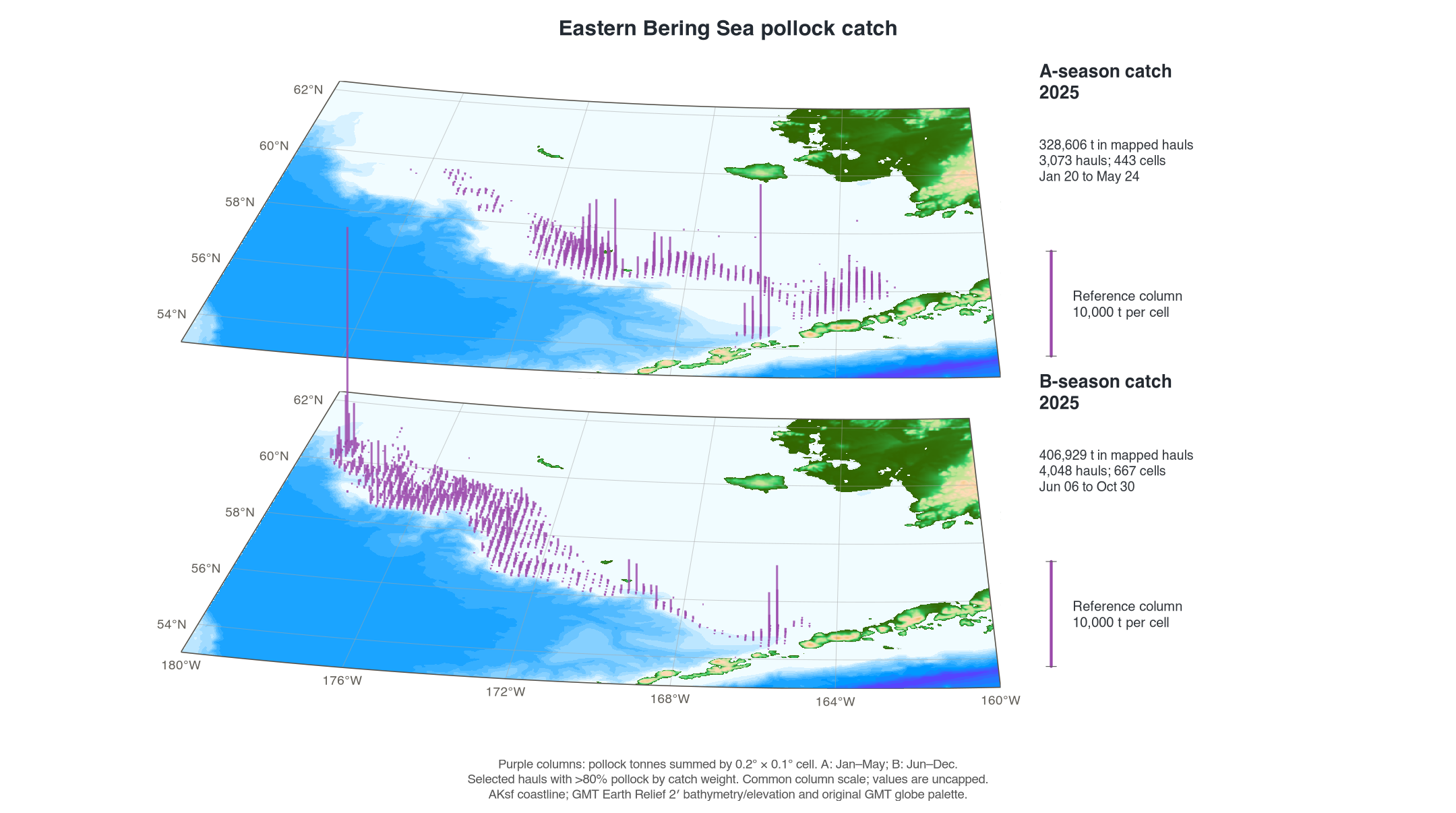
2025 and 2024

These oblique map planes retain the original GMT elevation palette and a common 10,000-tonne reference column. Their frame spans 180–160°W and 53–62.3°N. Use the reference column when comparing them with the 2026 terrain view, which has a different column scale and camera.

Eastern Bering Sea 2025 catch maps, with A season above B season. Purple columns show tonnes per geographic cell on the common 10,000-tonne reference scale; blue depth bands and green-to-tan land follow the historical GMT palette.

Open full-size figure

Eastern Bering Sea 2024 catch maps, with A season above B season. Purple columns show selected source-haul catch summed in 0.2 by 0.1 degree cells, using the same 10,000-tonne reference as the 2025 figure.

Open full-size figure

Experimental B-season view

This standalone 2026 B-season view retains a 36° viewing elevation, with the same 15× terrain exaggeration, 100 m land cap, azimuth, frame, and catch totals as the 2026 seasonal pair.

Experimental 2026 B-season eastern Bering Sea terrain view, with purple catch columns, 15-fold terrain exaggeration, land flattened above 100 metres, and a 36-degree viewing elevation. The catch extract is partial through 18 September.

Open full-size figure

Bathymetry source

The elevation raster comes from GMT Earth Relief, rather than AKsf. The saved maps use cached pixel-registered SRTM15+ Earth Relief v2.7 at 2 arc minutes, recorded in the local GMT catalog dated 1 May 2025, with a 10.5 km full-width Gaussian filter. Elevations are in metres. The raster was reprojected with bilinear interpolation to an approximately 2 km Alaska Albers display grid. The survey and 2024/2025 catch maps use the historical GMT palette; 2026 terrain maps add illumination and vertical exaggeration. Source elevations and catch totals retain their original values.

Grey 200 m and 500 m contour overlays and water-depth legends are omitted. Depth-color bands remain visible, including where survey values lack support. AKsf’s bundled Natural Earth coastline supplies generalized land geometry. See GMT’s Earth Relief documentation for the upstream grid product and download conventions.

Keep updates simple

For the production mapping project, keep each measurement in its own CSV with one record per row. Retain observed zeros; use NA for missing measurements. Keep dates, years, coordinates, units, and the source/correction version with the input. Do not fill unobserved ATS intervals with zeros.

Input	Columns used by the mapping project	Units
pollock.csv	year, lon, lat, cpue_kg_ha	kg/ha; ddc_cpue_kg_ha is the accepted source-column alias
temperature.csv	year, lon, lat, bottom_temp_c	°C; gear_temperature is the accepted source-column alias
avo.csv	year, lon, lat, sa	Sa source units; sA is an accepted alias
ATS spatial CSV	INTERVAL, region, lon, lat, biomass_ton, numbers_millions	t per EDSU and millions per EDSU; the configured year must match the interval identifiers
Fishery haul CSV	year, haul_date, lon, lat, nmfs_area, pollwt, official_total_catch	pollwt in kg; official_total_catch in t

The first three inputs also accept start_longitude and start_latitude. Supply one accepted name for each field. Fishery composition is checked after accounting for the kg/t unit difference.

1. Replace or append the CSV inputs in the mapping project, keeping existing years and the same columns.
2. Point config.R to the inputs; set the ATS year and fishery years as needed. The default annual-panel selection uses the latest eight available years with both CPUE and temperature.
3. Run Rscript run_maps.R from that project. If rebuilding AVO from the source track files, first run Rscript R/compile_avo.R.
4. Review the observation counts, missing values, catch-cell totals, date coverage, and source manifests before sharing the refreshed figures.

The production scripts and inputs are maintained outside AKsf; installing the package supplies the spatial geometry, not those application files. Updating this article is a separate documentation step. From the mapping project, sync the reviewed outputs to the package checkout and companion pollock wiki:

Show/hide shell code

python3 scripts/sync_map_docs.py --aksf /path/to/AKsf --wiki /path/to/pollock/wiki

The sync helper refreshes the selected figure assets and path-free manifests. Review the article’s snapshot date, years, and coverage text when the inputs change. Package vignette builds execute the synthetic example and display the archived figures; they do not rerun the source surveys or fishery analysis.