Mapping Alaska fisheries with AKsf

Show/hide R code

knitr::opts_chunk$set(collapse = FALSE, comment = "#>", fig.width = 7, fig.height = 5)
library(AKsf)
library(ggplot2)

AKsf uses the same building-block approach as nzsf: getters return sf objects, and plotters add geom_sf layers. The bundled snapshots make this tutorial work offline. Source definitions and derivations are documented in the repository’s DATA_SOURCES.md.

Show/hide R code

ggplot() +
  plot_reporting_areas(c("541", "542", "543"), fill = "#b5d9e8",
                        colour = "#345b6c", linewidth = 0.3) +
  plot_coast(fill = "grey88", colour = "grey50", linewidth = 0.15) +
  coord_aksf() + theme_aksf()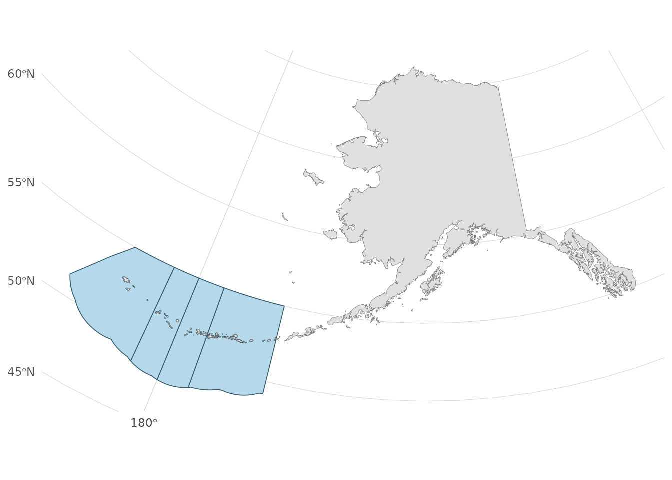

coord_aksf() and the default projected getters keep the western Aleutians near the rest of Alaska. A geographic longitude range can instead span nearly the entire world. Use the same CRS for data and analytical operations.

Plans and agency units

Show/hide R code

get_fmp_catalog()[, c("fmp_id", "plan_name")]

#>      fmp_id                                                         plan_name
#> 1   BSAI_GF Groundfish of the Bering Sea and Aleutian Islands Management Area
#> 2    GOA_GF                                  Groundfish of the Gulf of Alaska
#> 3 BSAI_CRAB             Bering Sea and Aleutian Islands King and Tanner Crabs
#> 4   SCALLOP                                        Scallop Fishery off Alaska
#> 5    SALMON                            Salmon Fisheries in the EEZ off Alaska
#> 6    ARCTIC                      Fish Resources of the Arctic Management Area

Show/hide R code

fmp <- get_fmp_areas(c("BSAI_GF", "GOA_GF"))
fmp[, c("fmp_id", "geometry_basis", "boundary_status")]

#> Simple feature collection with 2 features and 3 fields
#> Geometry type: MULTIPOLYGON
#> Dimension:     XY
#> Bounding box:  xmin: -2540688 ymin: 42347.24 xmax: 1360574 ymax: 1840526
#> Projected CRS: NAD83 / Alaska Albers
#>    fmp_id                                        geometry_basis
#> 1 BSAI_GF adfg_federal_areas_clipped_to_noaa_reporting_envelope
#> 2  GOA_GF adfg_federal_areas_clipped_to_noaa_reporting_envelope
#>                         boundary_status                       geometry
#> 1 cartographic_reference_not_regulatory MULTIPOLYGON (((-1722383 97...
#> 2 cartographic_reference_not_regulatory MULTIPOLYGON (((-1074317 42...

The six FMPs overlap across fisheries. Salmon has East, West, and Cook Inlet features. Crab extends eastward to Scotch Cap south of the Aleutians, whereas the BSAI groundfish boundary is farther west. These broad reference polygons do not describe stock boundaries, closures, or permission to fish.

Joining reporting areas to observations

Show/hide R code

observations <- data.frame(station = c("west", "central"),
                           longitude = c(-176, -172), latitude = c(52, 53))
points <- sf::st_as_sf(observations, coords = c("longitude", "latitude"), crs = 4326)
points <- sf::st_transform(points, proj_aksf())
areas <- get_reporting_areas(c("541", "542", "543"))
# Dissolve multipart source records by code before assigning a code to points.
by_code <- aggregate(areas["area_code"], by = list(code = areas$area_code), FUN = unique)
hits <- sf::st_intersects(points, by_code)
# Zero matches are outside coverage; multiple matches may lie on a boundary.
points$n_matches <- lengths(hits)
points$reporting_area <- vapply(hits, function(i) {
  if (length(i) == 1L) by_code$code[i] else NA_character_
}, character(1))
sf::st_drop_geometry(points)

#>   station n_matches reporting_area
#> 1    west         1            541
#> 2 central         1            541

Do not silently choose the first polygon for a boundary point. State-water areas and the Donut Hole are not interchangeable with U.S. federal FMP coverage.

ADF&G codes and provenance

Show/hide R code

registration <- get_registration_areas()
sf::st_drop_geometry(registration)[, c("area_code", "area_name")]

#>   area_code                        area_name
#> 1         K                      Kodiak Area
#> 2         M      South Alaska Peninsula Area
#> 3         O Bering Sea-Aleutian Islands Area
#> 4         Y            Chukchi-Beaufort Area
#> 5         L                     Chignik Area
#> 6         A      Eastern Gulf of Alaska Area
#> 7         E        Prince William Sound Area
#> 8         H                  Cook Inlet Area

Show/hide R code

# The complete six-digit groundfish statistical layer is also bundled:
# stat <- get_statistical_areas()
# federal <- stat[stat$WATERS_CODE == "FED", ]

Use character strings for joins with area codes. ADF&G’s native hierarchy and source date fields remain available. Groundfish polygons are not universal reporting grids for every fishery.

Show/hide R code

# A JSON manifest, readable without installing additional runtime packages.
cat(head(get_sources(), 10), sep = "\n")

#> [
#>   {
#>     "dataset": "nmfs_reporting_areas",
#>     "source_url": "https://alaskafisheries.noaa.gov/arcgis/rest/services/Base_Map/MapServer/0",
#>     "where": "1=1",
#>     "retrieved_utc": "2026-09-21T14:46:20.305706+00:00",
#>     "feature_count": 25,
#>     "output_crs": "EPSG:4326",
#>     "sha256": "e8a5c5483c12cc163938c53b0e4e54551d5348f0cec5156c126cf0e72095936d",
#>     "source_crs": {

Retrieval dates identify the snapshot, not when a boundary became legally effective. In particular, NOAA ATB’s salmon West source has a 2023 edit date; AKsf separates Cook Inlet following the 2024 plan but does not certify every source exclusion against later amendments. For regulatory work consult current NOAA, ADF&G, and NPFMC materials.