NOAA Alaska spatial closures: sources and mapping • AKsf

Show/hide R code

knitr::opts_chunk$set(collapse = FALSE, comment = "#>", fig.width = 8, fig.height = 5)
library(AKsf)
library(sf)
library(ggplot2)

Reviewed 2026-09-21, starting from NOAA’s Alaska fisheries portal. This vignette connects NOAA closure resources to AKsf maps. It includes an offline historical example, a service-discovery recipe, and GMT export. It does not provide a live open/closed decision for a vessel or fishery.

Find the right kind of restriction

Resource	What it helps you find	How to use it with AKsf
Habitat conservation area maps	Habitat restrictions, including gear-specific protection; PDF and GIS/mobile mapping resources	Overlay the relevant habitat layer on reporting or FMP areas.
Steller sea lion protection measures	Prey-fishery protections and links for Atka mackerel, Pacific cod trawl/non-trawl, pollock, and no-groundfish sites	Select the fishery and gear before selecting geometry.
Inseason fisheries management	Information bulletins, openings/closures, harvest specifications, and status reports	Treat temporal status as a separate source from the spatial boundary.
Status of fisheries	Groundfish status reports	Record the report date and applicable area, species, and sector.
Figures, maps, boundaries, areas, and zones	Cross-references to spatial products and regulatory figures	Identify the map and its underlying authority; do not equate every polygon with a closure.
Federal regulations and notices	The regulatory framework, including 50 CFR 679 and 680	Resolve the applicable rule, exceptions, and effective dates against the original material.

An FMP boundary describes management geography; it is not inherently a fishing closure. Likewise, essential fish habitat or critical habitat geometry alone does not encode a universal prohibition. A usable restriction record needs place, activity/gear, species or fishery, sector where applicable, time, and exceptions. Geometry is only one of those fields.

NOAA’s mapping index directs readers to regulations for official closure information. For current fishing decisions, follow those regulatory and inseason sources, not the teaching map below.

Inspect NOAA’s spatial service

The Alaska Regional Office Base_Map service exposes these polygon layers at the time of review:

Layer ID	Service name	Interpretation
0	`NMFS_Reporting_Areas`	Reporting geography, already substantially covered by AKsf.
1	`Atka_Mackerel`	Fishery-specific integrated spatial restrictions.
2	`PCod_Trawl`	Pacific cod trawl restriction geography.
3	`Pcod_Non_Trawl`	Pacific cod non-trawl restriction geography.
4	`Pollock`	Pollock restriction geography.
5	`Habitat_Restrictions`	Habitat/restriction composite used for the example below.
6	`SSL_CH`	Steller sea lion critical habitat context.
7	`SSL_Zones`	Steller sea lion zones; inspect attributes and linked rules before interpretation.

Layer IDs belong to this service, not to a universal NOAA catalog. Inspect the service before reusing an ID. Fields are not standardized across the layers: for example, layer 4 uses lowercase htm, while layer 5 uses HTM. OBJECTID is a service feature identifier, not a durable regulatory area code.

The Spatial Management Areas metadata describes an integrated product where overlapping restrictions were processed in a hierarchy. Consequently, a composite feature need not reproduce the full original footprint of every contributing measure. Do not combine the fishery composites and habitat layer and count their areas as independent restrictions. For totals across overlapping polygons, first define the applicable rule set, then decide whether a union or separate rule-specific totals answer the question.

Check vintage before mapping

The selected records in Habitat_Restrictions have dtd = "steve.lewis, akro, 01/19/15". The layer metadata did not expose an editingInfo timestamp when inspected. A website update date, retrieval date, or new download does not establish a new legal effective date. Here dtd is retained as a source annotation, not interpreted as a legal validity interval.

The sample contains just two source records: GOA_Slope_HCA.htm and GOA_Coral_HPA.htm. Those records can contain multiple polygon components. They are a historical teaching example, not a comprehensive closure inventory or certification of the current GOA restrictions.

Load the pinned example without a network connection

Show/hide R code

example_dir <- system.file("extdata", "closure-example", package = "AKsf")
closures <- st_read(file.path(example_dir, "goa-habitat.geojson"), quiet = TRUE)
manifest <- jsonlite::fromJSON(file.path(example_dir, "manifest.json"))
stopifnot(nrow(closures) == manifest$feature_count,
          setequal(closures$OBJECTID, manifest$object_ids),
          !any(st_is_empty(closures)))
knitr::kable(st_drop_geometry(closures)[, c("OBJECTID", "HTM", "dtd")])

OBJECTID	HTM	dtd
12	GOA_Slope_HCA.htm	steve.lewis, akro, 01/19/15
15	GOA_Coral_HPA.htm	steve.lewis, akro, 01/19/15

The accompanying manifest records the service/query URL, object IDs, retrieval time, SHA-256 checksum, and source annotation. Raw geometry and attributes are retained as supplied by NOAA, with the service asked to return EPSG:4326. The example is separate from AKsf’s main data catalog and FMP reference layers.

Map closures as a separate layer

Transform before spatial operations. Keep the source object for traceability; any validity repair below applies to the mapping copy.

Show/hide R code

closure_map <- st_transform(closures, proj_aksf())
if (!all(st_is_valid(closure_map))) closure_map <- st_make_valid(closure_map)
labels <- c(GOA_Slope_HCA.htm = "GOA slope habitat conservation",
            GOA_Coral_HPA.htm = "GOA coral habitat protection")
closure_map$map_label <- unname(labels[closure_map$HTM])
bb <- st_bbox(closure_map)
pad <- 100000 # metres in EPSG:3338

ggplot() +
  plot_fmp_areas("GOA_GF", fill = "#e8f1f5", colour = "#7896a5", linewidth = 0.25) +
  plot_reporting_areas(fill = NA, colour = "grey70", linewidth = 0.2) +
  geom_sf(data = closure_map, aes(fill = map_label), colour = "#6e2745", linewidth = 0.5) +
  plot_coast(fill = "grey90", colour = "grey60", linewidth = 0.2) +
  scale_fill_manual(NULL, values = c("#d88b54", "#9e77b4")) +
  coord_aksf(xlim = c(bb["xmin"] - pad, bb["xmax"] + pad),
             ylim = c(bb["ymin"] - pad, bb["ymax"] + pad), expand = FALSE) +
  theme_aksf() +
  theme(legend.position = "bottom", legend.text = element_text(size = 9)) +
  labs(title = "Selected GOA habitat restriction footprints",
       subtitle = "Historical GIS example • source annotation 2015",
       caption = "NOAA AKRO geometry • AKsf FMP reference • Natural Earth land")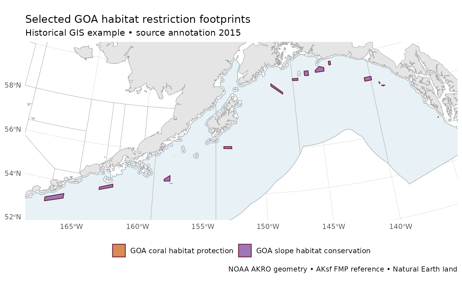

Historical NOAA GIS example: selected GOA habitat records, source annotation 2015; retrieved 2026-09-21. This is not a current closure-status map.

The pale FMP background supplies context only. The map does not infer that unshaded water is open or that all fishing is prohibited inside colored areas. The service’s Shape_Area values are source attributes; for a spatial analysis, calculate area from an appropriate equal-area geometry instead of treating Web Mercator area values as geodesic area.

Use the same example in GMT

Show/hide R code

gmt_file <- tempfile(fileext = ".gmt")
write_gmt(closure_map[, c("OBJECTID", "HTM", "dtd")], gmt_file)
stopifnot(file.exists(gmt_file))
unlink(gmt_file)

For a persistent output, replace gmt_file with "goa-habitat-example.gmt". Use gmt plot goa-habitat-example.gmt within the map session described in the GMT vignette. Preserve the source-vintage label on the GMT figure. Changing the output format does not change the meaning or currency of the data.

Discover or refresh source data deliberately

This optional block inspects the service online; it is not executed during package or website builds:

Show/hide R code

service <- "https://alaskafisheries.noaa.gov/arcgis/rest/services/Base_Map/MapServer"
catalog <- jsonlite::fromJSON(paste0(service, "?f=pjson"))
if (!is.null(catalog$error)) stop(catalog$error$message)
catalog$layers[, c("id", "name")]

metadata <- jsonlite::fromJSON(paste0(service, "/5?f=pjson"))
if (!is.null(metadata$error)) stop(metadata$error$message)
metadata$fields[, c("name", "type")]
metadata$editingInfo # Absence is not evidence of currency.

The repository’s data-raw/download-closure-example.py rebuilds the two-record snapshot. It first queries matching object IDs, requests those geometries, checks that every requested ID was returned, and saves metadata and a checksum. For larger layer downloads, batch the ID list within service limits and verify completeness; a single successful response can still be truncated. Keep the original data alongside any transformed, repaired, or simplified derivative. Review changed geometry and source notes before replacing a published snapshot.

For a time-specific study, record the observation date, species, gear, sector, source revision, and applicable notices with each analysis. Do not fill absent season/exception fields by guessing from a layer name or an HTM filename. The .htm tokens in this service are retained identifiers, not guaranteed live URLs or substitutes for the linked regulatory text.

Relation to the other Alaska packages

Use akgfmaps for survey design and strata, coldpool for environmental products, and AKsf for FMP/reporting context. A closure polygon is not a survey stratum. navmaps can format operational layers, but this historical example should not be promoted to a current navigation layer. Maintain the NOAA restriction source and date independently from each package’s basemap version.