Seasonal and Size-Related Patterns in Pollock Sex Ratio and Growth

Author

Jim Ianelli

Published

August 4, 2026

1 Overview

This report presents an exploratory analysis of pollock fishery age data from the Gulf of Alaska (GOA) and Bering Sea and Aleutian Islands (BSAI), along with complementary acoustic-survey summaries. Its purpose is to identify seasonal, size-related, spatial, and interannual patterns in sex ratio and growth that may warrant further investigation; the results should not be interpreted as a formal assessment-model test.

Explore seasonal length-frequency patterns

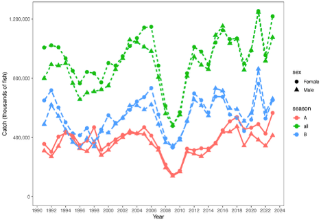
These data are parsed using the R code presented below and cover 1986-2025, with the A-season catcher/processor weekly summaries updated through 2026. Figure 1 provides context for sex-specific differences in fishery catch prior to the age and length analyses based on appropriately raised estimates of catch-at-age by sex and season (Ianelli et al. 2024). The figure indicates slight variability in sex-specific structure in catch across years but without a strong indication that the sex-ratio deviates consistently from year to year. These patterns motivate explicit sex-specific summaries in the subsequent age- and length-based diagnostics.

Time series of EBS pollock catch by female and male fish across A season, B season, and total catch.
Figure 1: Estimated EBS pollock catch numbers by sex for the A season (January-May), B season (June-October), and total. Source: Ianelli et al. (2024).
Show code
filter_plot_data <- function(data, season_filter = NULL, fmp_filter = NULL) {
  data <- data %>%
    filter(SEX %in% c("F", "M"))

  if (!is.null(season_filter)) {
    data <- data %>%
      filter(season %in% season_filter)
  }

  if (!is.null(fmp_filter)) {
    data <- data %>%
      filter(fmp %in% fmp_filter)
  }

  data
}

summarize_sex_ratio <- function(data, group_vars) {
  data %>%
    group_by(!!!group_vars) %>%
    summarize(
      female_n = sum(SEX == "F"),
      male_n = sum(SEX == "M"),
      total_n = female_n + male_n,
      sex_ratio = female_n / total_n,
      .groups = "drop"
    )
}

build_facet_vars <- function(primary_facet = NULL, facet_season = FALSE, facet_fmp = FALSE) {
  facet_vars <- list()

  if (!is.null(primary_facet) && !rlang::quo_is_null(primary_facet)) {
    facet_vars <- c(facet_vars, list(primary_facet))
  }

  if (facet_season) {
    facet_vars <- c(facet_vars, rlang::quos(season))
  }

  if (facet_fmp) {
    facet_vars <- c(facet_vars, rlang::quos(fmp))
  }

  facet_vars
}

plot_sex_ratio <- function(data, x_var, facet_var = NULL, min_n = 5,
                           y_limits = c(0.3, 0.7), show_labels = FALSE,
                           facet_ncol = 6, season_filter = NULL,
                           fmp_filter = NULL, facet_season = FALSE,
                           facet_fmp = FALSE, color_var = NULL) {
  x_var <- rlang::enquo(x_var)
  facet_var <- rlang::enquo(facet_var)
  facet_vars <- build_facet_vars(facet_var, facet_season = facet_season, facet_fmp = facet_fmp)
  color_sym <- if (is.null(color_var)) NULL else rlang::sym(color_var)
  group_vars <- c(facet_vars, list(x_var), if (is.null(color_sym)) list() else list(color_sym))

  plot_df <- data %>%
    filter_plot_data(season_filter = season_filter, fmp_filter = fmp_filter) %>%
    summarize_sex_ratio(group_vars) %>%
    filter(total_n >= min_n)

  plot_mapping <- aes(x = !!x_var, y = sex_ratio)
  if (!is.null(color_sym)) {
    plot_mapping$colour <- color_sym
  }
  color_label <- if (is.null(color_var)) {
    NULL
  } else {
    dplyr::case_match(
      color_var,
      "season" ~ "Season",
      "fmp" ~ "FMP",
      .default = color_var
    )
  }

  p <- ggplot(plot_df, plot_mapping)

  if (show_labels) {
    p <- p +
      geom_text(
        aes(label = round(total_n / 100, 1)),
        size = 2.8,
        alpha = 0.8,
        check_overlap = TRUE
      )
  } else {
    p <- p +
      geom_point(aes(size = total_n), alpha = 0.6)
  }

  p <- p +
    geom_smooth(method = "loess", formula = "y ~ x") +
    geom_hline(yintercept = 0.5, linetype = "dashed", color = "gray50") +
    scale_y_continuous(labels = scales::percent) +
    coord_cartesian(ylim = y_limits) +
    labs(
      title = paste("Sex Ratio (Proportion Female) by", rlang::as_label(x_var)),
      subtitle = if (show_labels) "Labels show Sample Size / 100" else "Points sized by sample size",
      x = rlang::as_label(x_var),
      y = "Sex Ratio",
      size = "Sample Size",
      color = color_label
    ) +
    theme_minimal(base_size = 11)

  if (length(facet_vars) > 0) {
    p <- p + facet_wrap(vars(!!!facet_vars), ncol = facet_ncol)
  }

  p
}

plot_sex_ratio_age_box <- function(data, min_n = 25, y_limits = c(0.3, 0.7),
                                   facet_ncol = 6, season_filter = NULL,
                                   fmp_filter = NULL, facet_season = FALSE,
                                   facet_fmp = FALSE) {
  facet_vars <- build_facet_vars(facet_season = facet_season, facet_fmp = facet_fmp)
  group_vars <- c(facet_vars, rlang::quos(age_group))

  plot_df <- data %>%
    filter_plot_data(season_filter = season_filter, fmp_filter = fmp_filter) %>%
    mutate(
      age_group = if_else(AGE > 13, "13+", as.character(AGE))
    ) %>%
    summarize_sex_ratio(group_vars) %>%
    filter(total_n >= min_n)

  numeric_ages <- suppressWarnings(as.integer(plot_df$age_group[plot_df$age_group != "13+"]))
  age_levels <- c(
    as.character(sort(unique(numeric_ages[!is.na(numeric_ages)]))),
    if (any(plot_df$age_group == "13+")) "13+" else character(0)
  )
  plot_df <- plot_df %>%
    mutate(
      age_group = factor(age_group, levels = age_levels),
      age_num = if_else(age_group == "13+", 13, as.numeric(as.character(age_group)))
    )

  p <- ggplot(plot_df, aes(x = age_num, y = sex_ratio)) +
    geom_point(aes(size = total_n), alpha = 0.5) +
    geom_smooth(method = "loess", formula = "y ~ x") +
    geom_hline(yintercept = 0.5, linetype = "dashed", color = "gray50") +
    scale_y_continuous(labels = scales::percent) +
    coord_cartesian(ylim = y_limits) +
    scale_x_continuous(
      breaks = c(as.integer(age_levels[age_levels != "13+"]), if ("13+" %in% age_levels) 13 else numeric(0)),
      labels = age_levels
    ) +
    labs(
      x = "Age (13+ pooled)",
      y = "Sex Ratio",
      size = "Sample Size"
    ) +
    theme_minimal(base_size = 11)

  if (length(facet_vars) > 0) {
    p <- p + facet_wrap(vars(!!!facet_vars), ncol = facet_ncol)
  }

  p
}

plot_sex_ratio_length_box <- function(data, bin_width = 5, min_n = 50,
                                      y_limits = c(0.3, 0.7), facet_ncol = 6,
                                      season_filter = NULL, fmp_filter = NULL,
                                      facet_season = FALSE, facet_fmp = FALSE) {
  facet_vars <- build_facet_vars(facet_season = facet_season, facet_fmp = facet_fmp)
  group_vars <- c(facet_vars, rlang::quos(length_bin_lower))

  plot_df <- data %>%
    filter_plot_data(season_filter = season_filter, fmp_filter = fmp_filter) %>%
    filter(LENGTH >= 20, LENGTH <= 65) %>%
    mutate(
      length_bin_lower = pmin(floor((LENGTH - 20) / bin_width) * bin_width + 20, 60)
    ) %>%
    summarize_sex_ratio(group_vars) %>%
    filter(total_n >= min_n) %>%
    mutate(
      length_bin_mid = if_else(length_bin_lower == 60, 62.5, length_bin_lower + bin_width / 2),
      length_bin = if_else(
        length_bin_lower == 60,
        "60-65",
        paste0(length_bin_lower, "-", length_bin_lower + (bin_width - 1))
      ),
      length_bin = factor(length_bin, levels = unique(length_bin[order(length_bin_lower)]))
    )

  p <- ggplot(plot_df, aes(x = length_bin_mid, y = sex_ratio)) +
    geom_point(aes(size = total_n), alpha = 0.5) +
    geom_smooth(method = "loess", formula = "y ~ x") +
    geom_hline(yintercept = 0.5, linetype = "dashed", color = "gray50") +
    scale_y_continuous(labels = scales::percent) +
    coord_cartesian(ylim = y_limits) +
    scale_x_continuous(
      breaks = unique(plot_df$length_bin_mid[order(plot_df$length_bin_lower)]),
      labels = unique(plot_df$length_bin[order(plot_df$length_bin_lower)])
    ) +
    labs(
      x = "Length Bin (cm, 20-65)",
      y = "Sex Ratio",
      size = "Sample Size"
    ) +
    theme_minimal(base_size = 11) +
    theme(axis.text.x = element_text(angle = 45, hjust = 1))

  if (length(facet_vars) > 0) {
    p <- p + facet_wrap(vars(!!!facet_vars), ncol = facet_ncol)
  }

  p
}

plot_mean_length_age_sex <- function(data, age_range = 2:10, facet_ncol = 6,
                                     season_filter = NULL, fmp_filter = NULL,
                                     facet_season = FALSE, facet_fmp = FALSE,
                                     facet_sex = FALSE, color_var = "sex",
                                     shape_var = NULL, facet_rows = NULL,
                                     facet_cols = NULL, linetype_var = NULL) {
  facet_names <- c(
    if (facet_season) "season",
    if (facet_fmp) "fmp",
    if (facet_sex) "sex"
  )
  facet_grid_names <- c(facet_rows, facet_cols)
  group_names <- unique(c(facet_names, facet_grid_names, "age_num", "sex", color_var, shape_var, linetype_var))

  plot_df <- data %>%
    filter_plot_data(season_filter = season_filter, fmp_filter = fmp_filter) %>%
    filter(!is.na(AGE), !is.na(LENGTH)) %>%
    mutate(
      age_num = as.numeric(AGE),
      sex = recode(SEX, F = "Female", M = "Male")
    ) %>%
    filter(age_num >= min(age_range), age_num <= max(age_range)) %>%
    group_by(across(all_of(group_names))) %>%
    summarize(
      mean_length = mean(LENGTH, na.rm = TRUE),
      .groups = "drop"
    )

  plot_mapping <- aes(x = age_num, y = mean_length)
  plot_mapping$colour <- rlang::sym(color_var)

  if (!is.null(shape_var)) {
    plot_mapping$shape <- rlang::sym(shape_var)
  }

  if (!is.null(linetype_var)) {
    plot_mapping$linetype <- rlang::sym(linetype_var)
  }

  line_group_names <- unique(c(color_var, shape_var, linetype_var, if (!facet_sex) "sex"))
  plot_mapping$group <- rlang::expr(interaction(!!!rlang::syms(line_group_names), drop = TRUE))
  color_label <- dplyr::case_match(
    color_var,
    "sex" ~ "Sex",
    "season" ~ "Season",
    "fmp" ~ "FMP",
    .default = color_var
  )
  shape_label <- if (is.null(shape_var)) {
    NULL
  } else {
    dplyr::case_match(
      shape_var,
      "sex" ~ "Sex",
      "season" ~ "Season",
      "fmp" ~ "FMP",
      .default = shape_var
    )
  }
  linetype_label <- if (is.null(linetype_var)) {
    NULL
  } else {
    dplyr::case_match(
      linetype_var,
      "sex" ~ "Sex",
      "season" ~ "Season",
      "fmp" ~ "FMP",
      .default = linetype_var
    )
  }

  p <- ggplot(plot_df, plot_mapping) +
    geom_point(size = 2.4, alpha = 0.9) +
    geom_smooth(method = "loess", formula = "y ~ x", se = FALSE, linewidth = 1.1) +
    scale_x_continuous(breaks = age_range) +
    labs(
      x = "Age",
      y = "Mean Length",
      color = color_label,
      shape = shape_label,
      linetype = linetype_label
    ) +
    theme_minimal(base_size = 11)

  if (!is.null(facet_rows) || !is.null(facet_cols)) {
    row_vars <- if (is.null(facet_rows)) list(.) else rlang::syms(facet_rows)
    col_vars <- if (is.null(facet_cols)) list(.) else rlang::syms(facet_cols)
    p <- p + facet_grid(rows = vars(!!!row_vars), cols = vars(!!!col_vars))
  } else if (length(facet_names) > 0) {
    p <- p + facet_wrap(vars(!!!rlang::syms(facet_names)), ncol = facet_ncol)
  }

  p
}
2 Exploratory figures

2.1 Fishery data

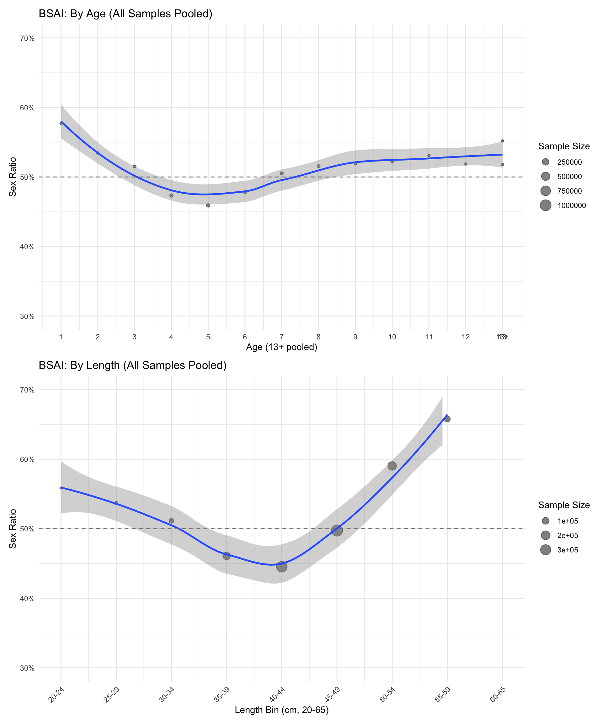
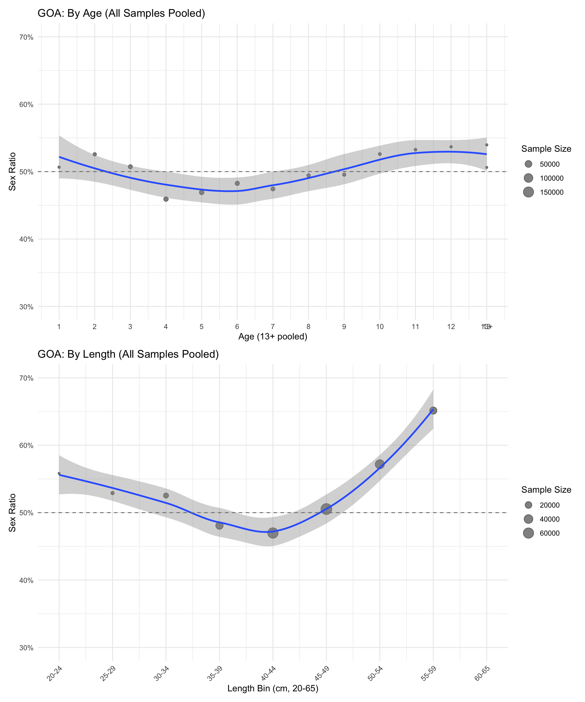
The exploratory sequence begins with pooled summaries that establish the overall relationship between sex ratio and fish size. The GOA view in Figure 2 and the BSAI view in Figure 3 each show sex ratio first by age and then by 5-cm length bin. These figures provide broad regional benchmarks before the data are separated by year, season, or subarea.

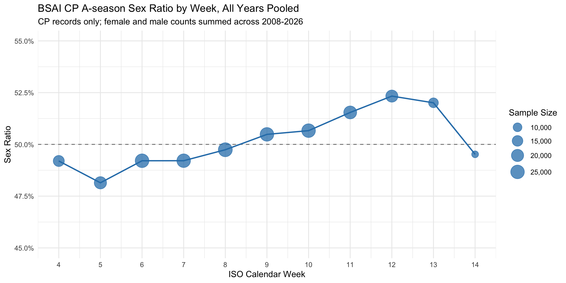
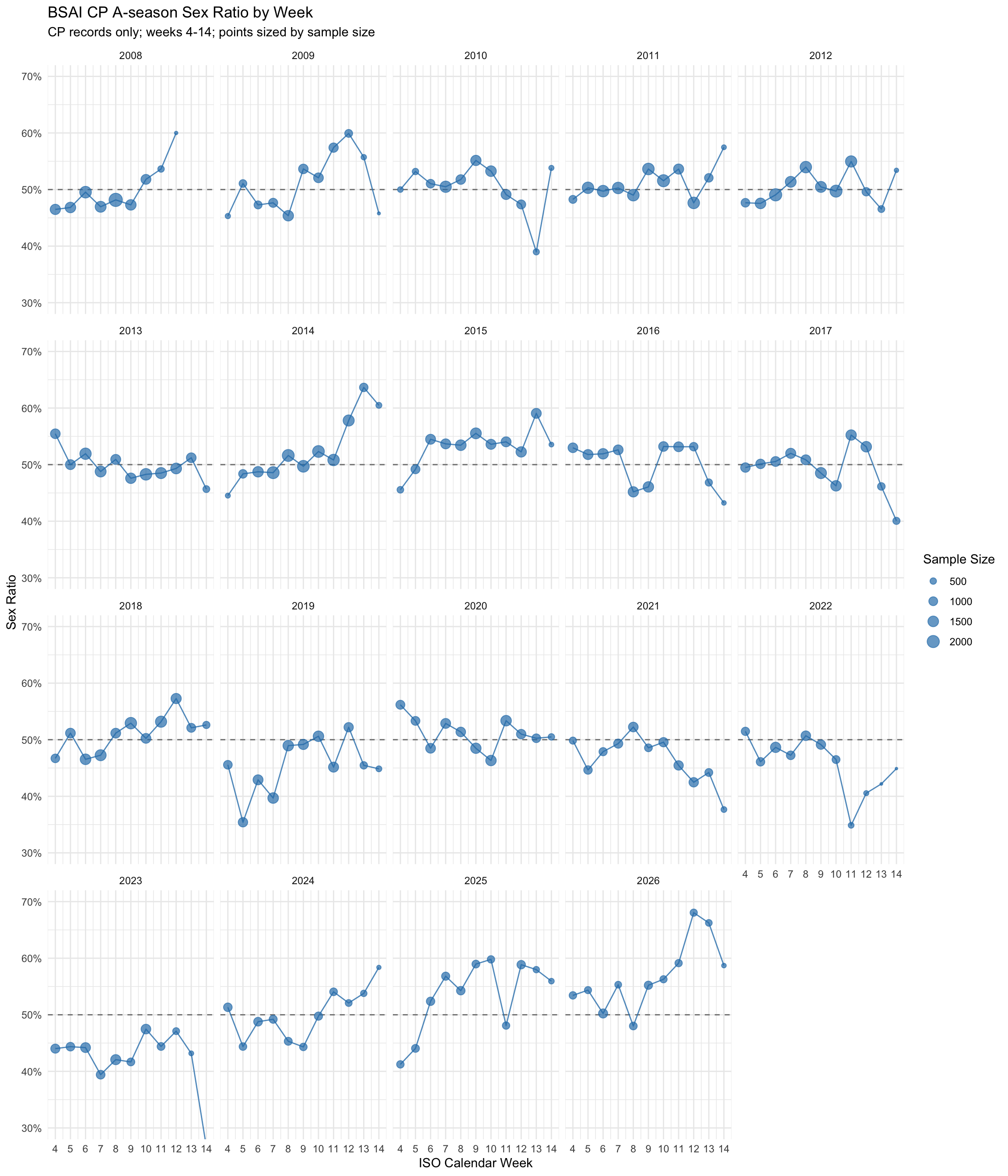
The next two figures focus on progression within the A season for the BSAI catcher/processor fleet. The annual-panel appendix (Figure 14) shows the sex ratio for ISO weeks 4-14 separately by year, making interannual differences in the within-season pattern visible. Figure 4 then pools female and male counts across all available years to show the overall weekly pattern. Both figures use CP records only, and point size indicates the number of fish contributing to each estimate.

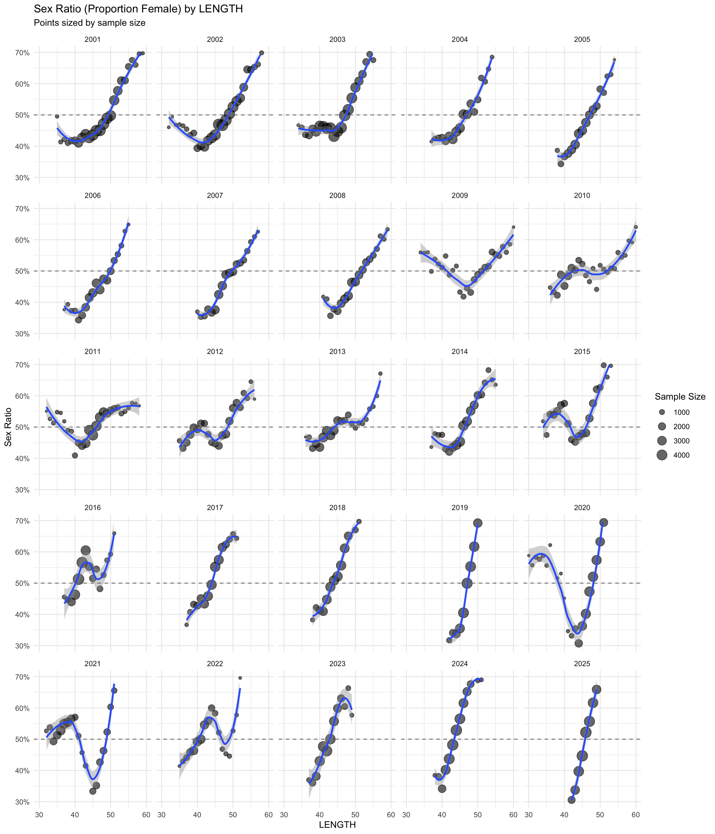
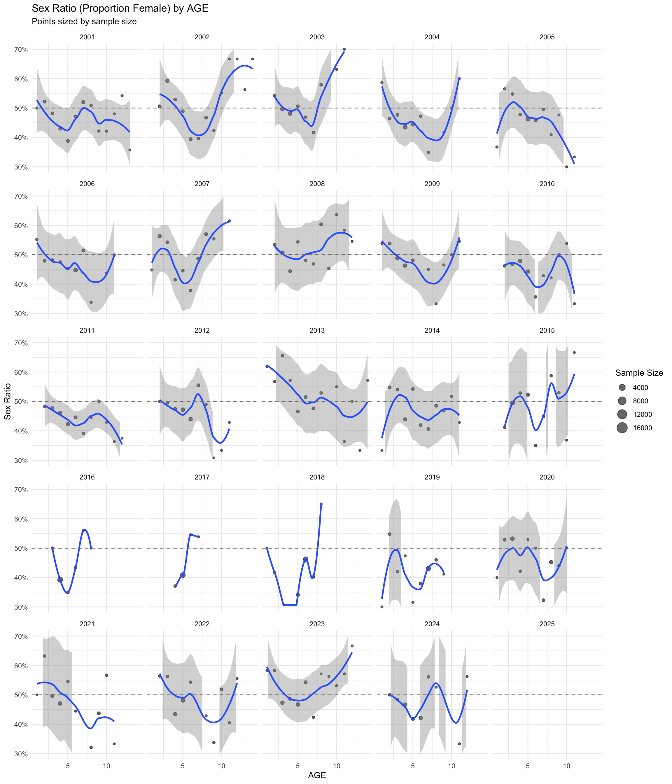
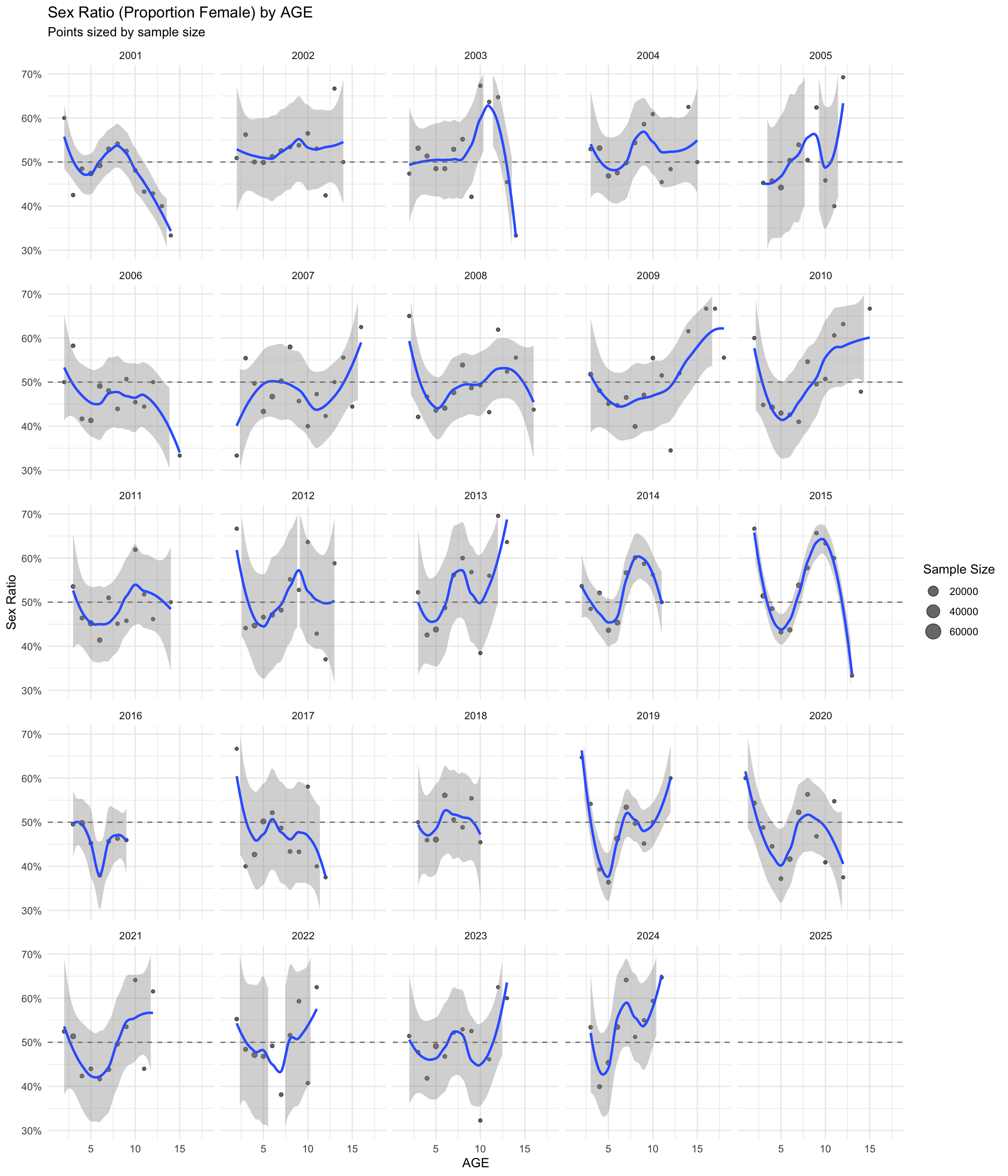
The analysis then shifts to interannual patterns in length and age. The annual-panel appendix provides length-based sex ratios by year for GOA in Figure 15 and for BSAI in Figure 16. The corresponding age-based views are shown in Figure 17 and Figure 18. Together, these figures show whether the pooled relationships persist across years or are driven by a smaller number of annual samples.

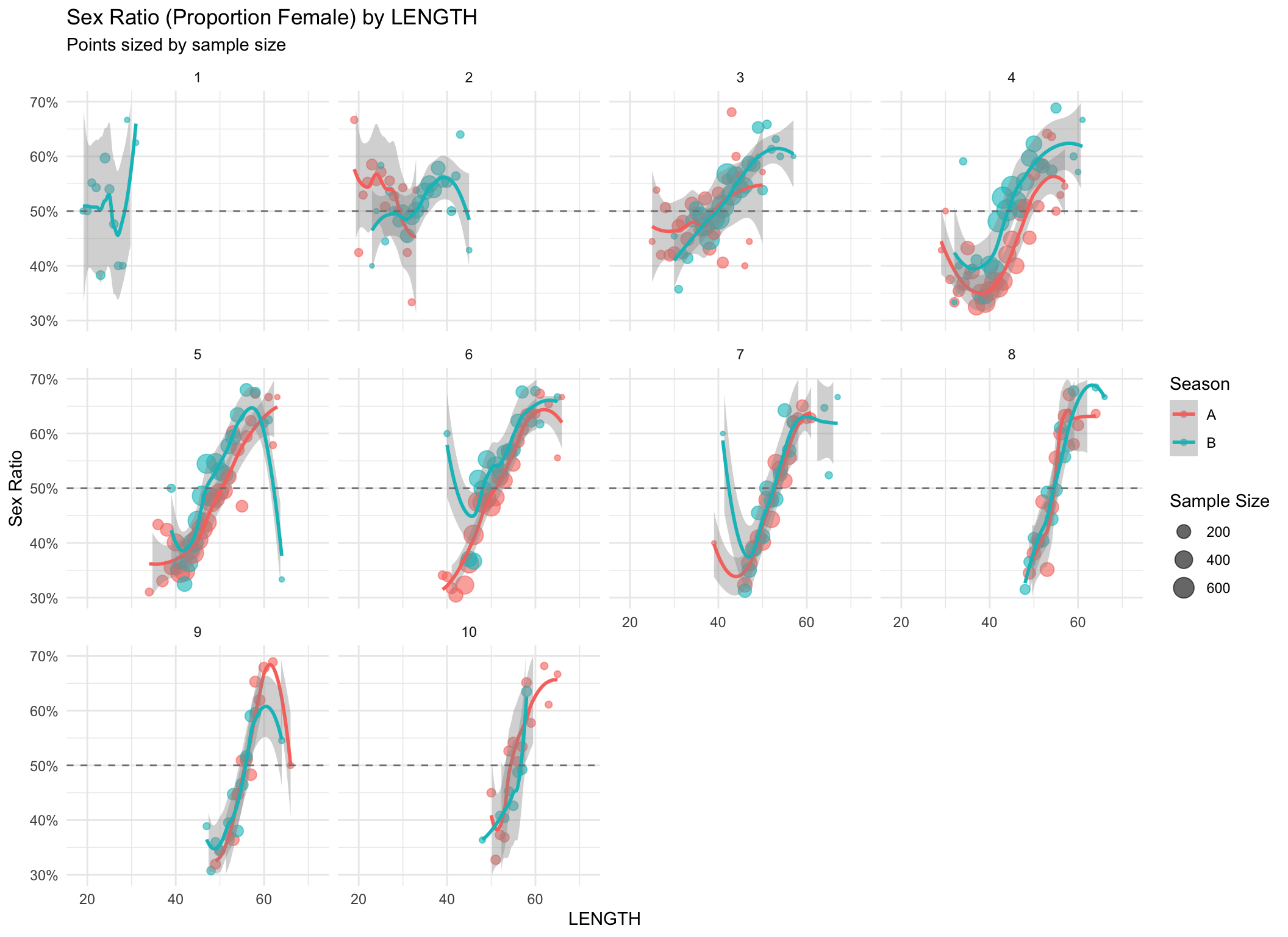
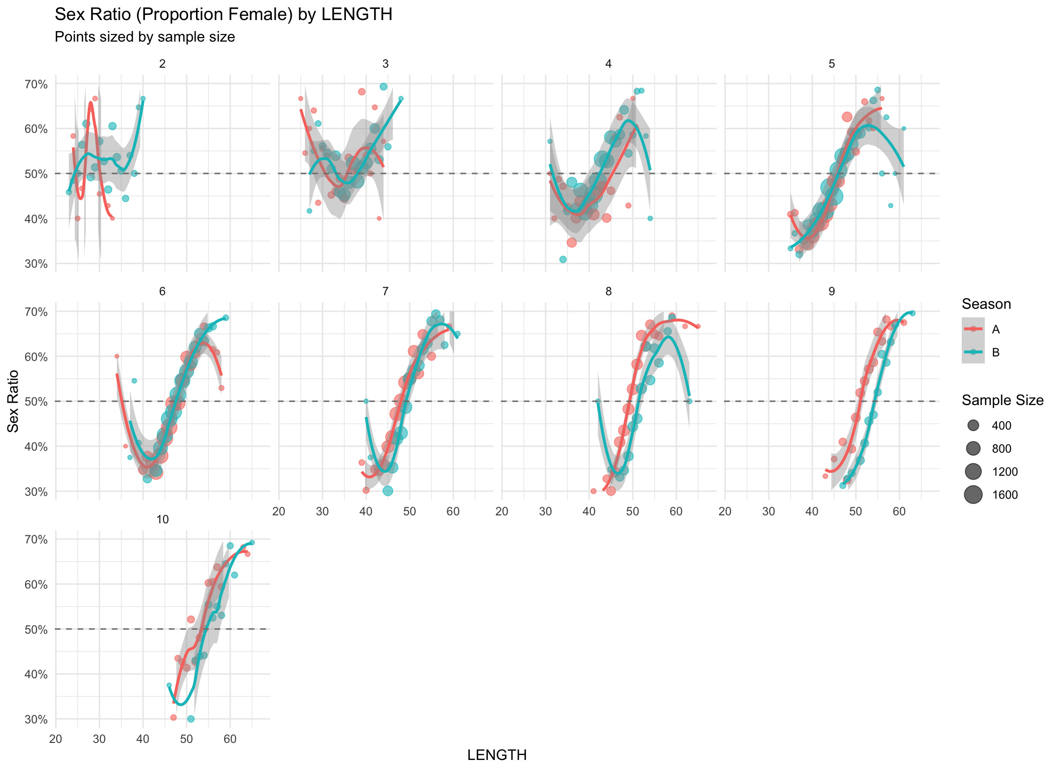
The next pair of figures reverses the perspective by faceting length-based sex ratios by age and displaying season as a separate series. The GOA results are shown in Figure 5 and the BSAI results in Figure 6. The seasonal pattern is broadly similar between regions, although the age-4 panels suggest that fish sampled during the A season tend to be slightly larger than those sampled during the B season, which is somewhat counterintuitive.

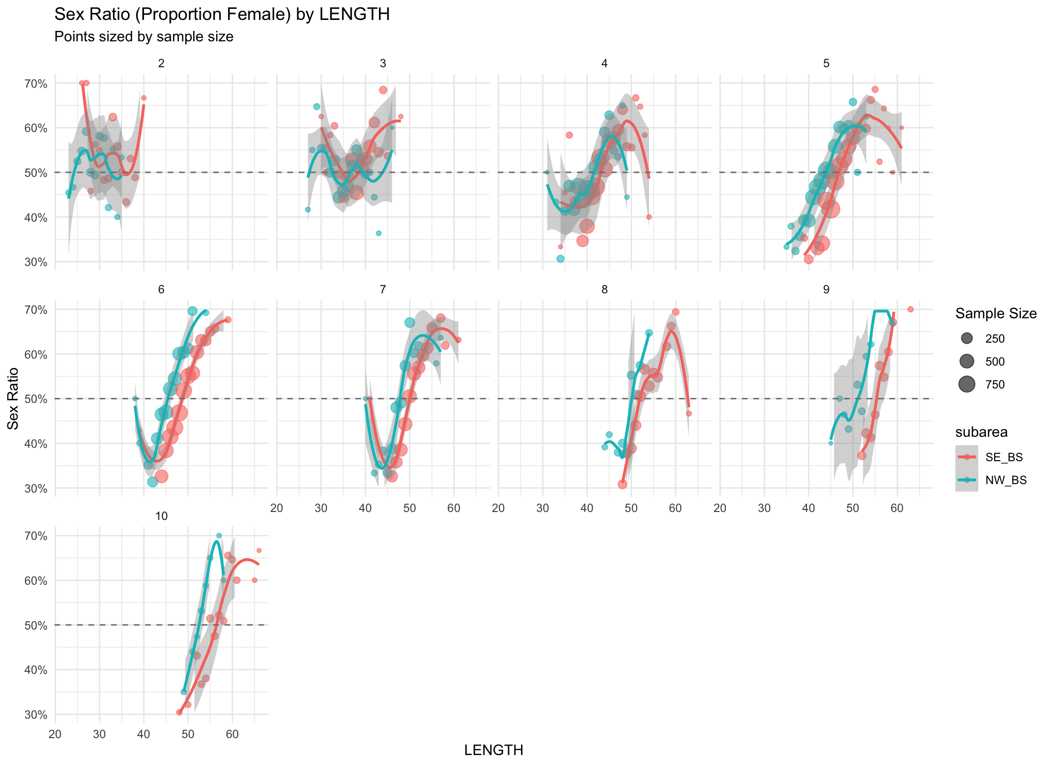
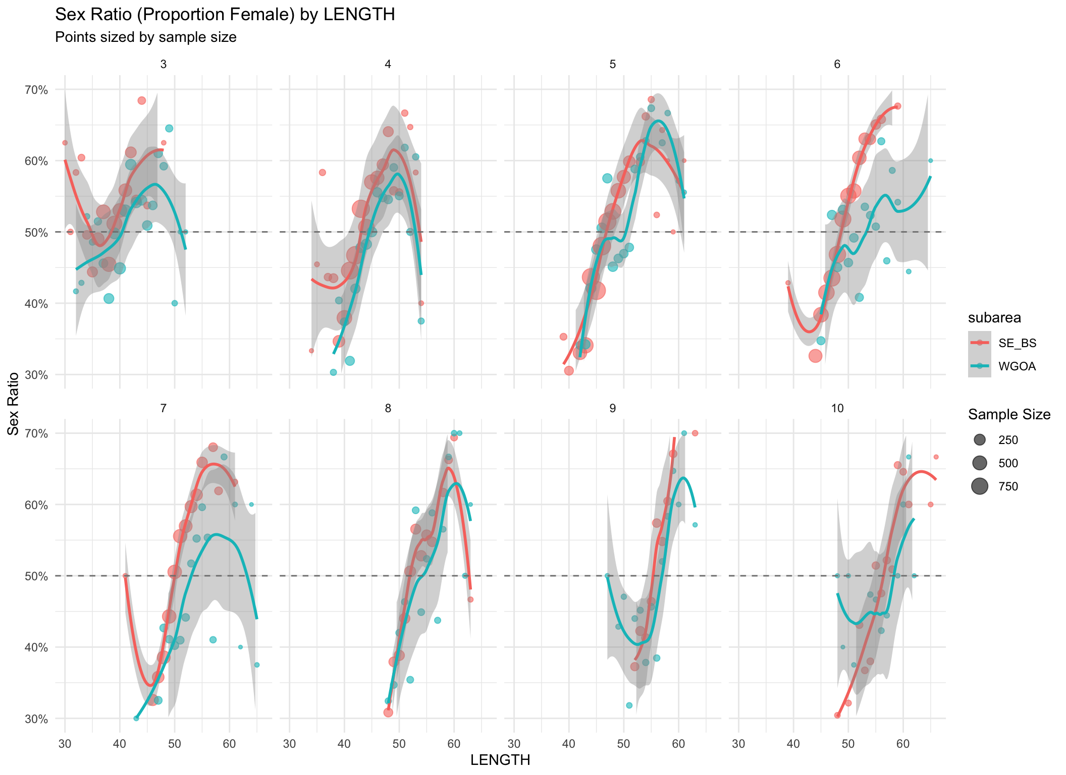
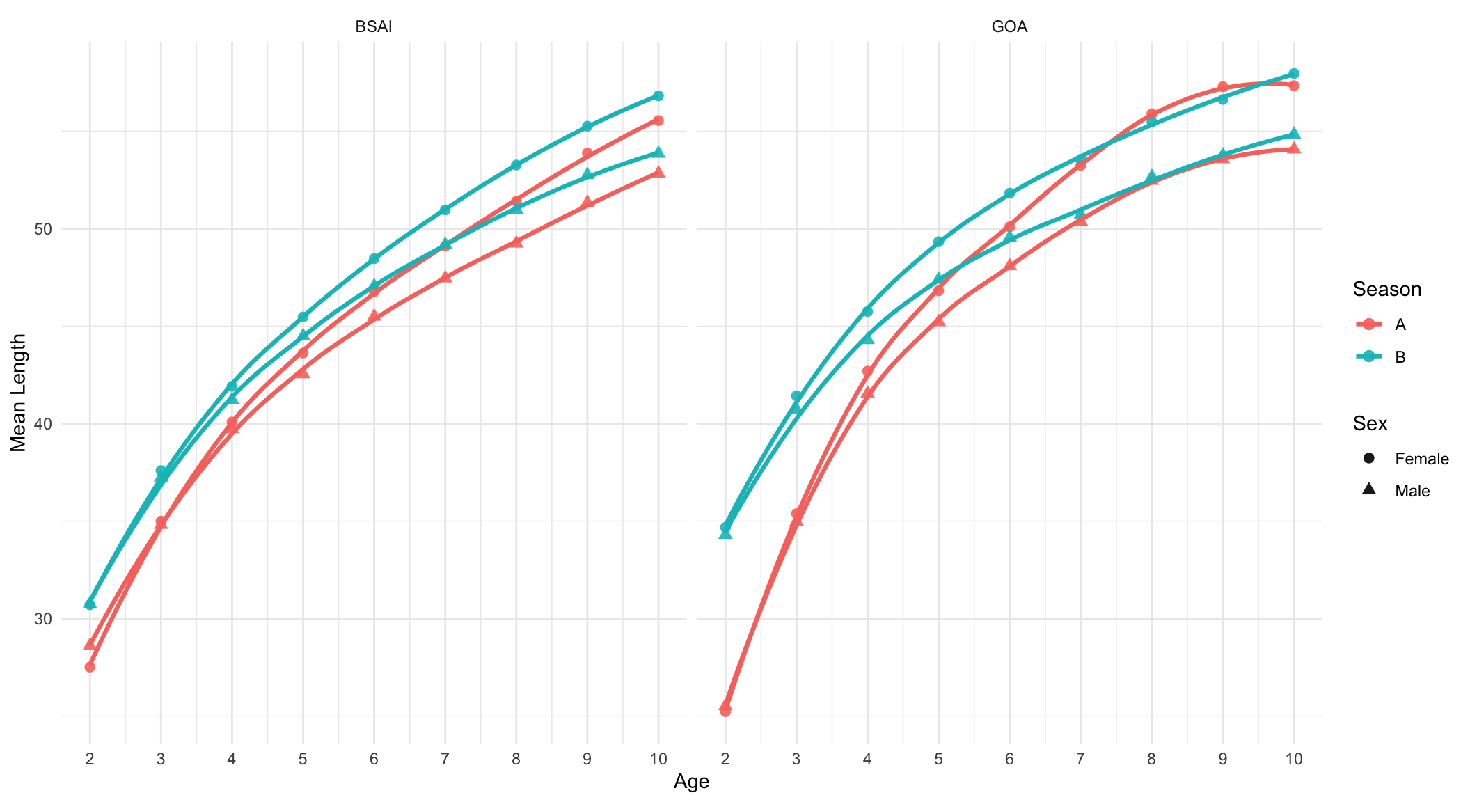
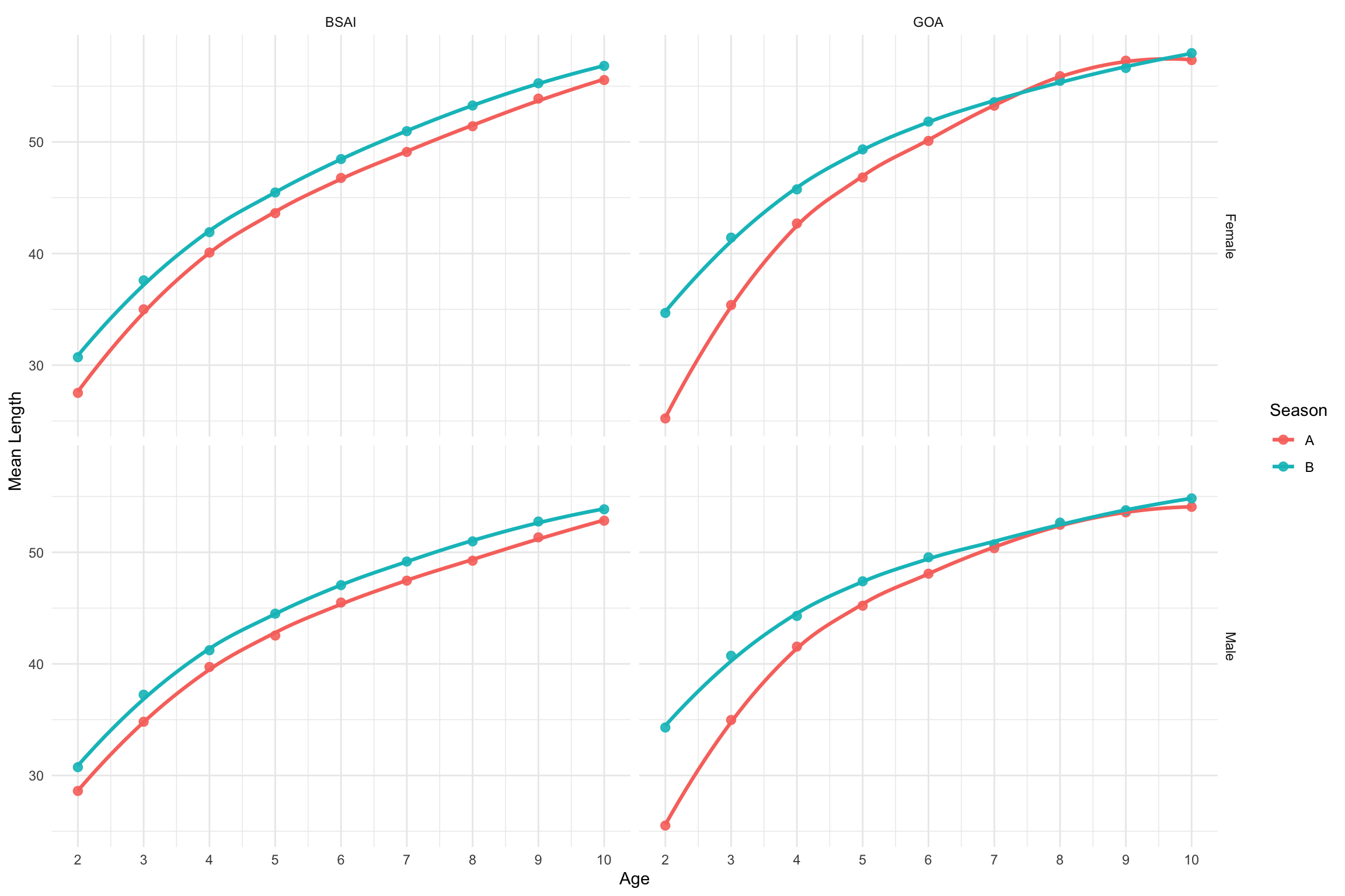
The final sex-ratio comparisons narrow the data by subarea. Figure 7 compares SE_BS with NW_BS during Season B, while Figure 8 compares SE_BS with WGOA for ages 3-10 during Season B. The exploratory sequence concludes with mean length-at-age summaries: Figure 9 separates the fishery management programs, seasons, and sexes, and Figure 10 provides the complementary layout with sex in rows and fishery management program in columns.

Show code
p_age_overall <- plot_sex_ratio_age_box(df_age, min_n = 25, fmp_filter = "GOA") +
  labs(title = "GOA: By Age (All Samples Pooled)")

p_length_overall <- plot_sex_ratio_length_box(df_age, bin_width = 5, min_n = 50, fmp_filter = "GOA") +
  labs(title = "GOA: By Length (All Samples Pooled)")

p_age_overall / p_length_overall + patchwork::plot_layout(heights = c(1, 1))
Figure 2: GOA pooled sex ratios across all samples: by age with ages >13 pooled to 13+ (top) and by 5-cm length bins for lengths 20-65 cm (bottom).
Show code
p_age_overall <- plot_sex_ratio_age_box(df_age, min_n = 25, fmp_filter = "BSAI") +
  labs(title = "BSAI: By Age (All Samples Pooled)")

p_length_overall <- plot_sex_ratio_length_box(df_age, bin_width = 5, min_n = 50, fmp_filter = "BSAI") +
  labs(title = "BSAI: By Length (All Samples Pooled)")

p_age_overall / p_length_overall + patchwork::plot_layout(heights = c(1, 1))
Figure 3: BSAI pooled sex ratios across all samples: by age with ages >13 pooled to 13+ (top) and by 5-cm length bins for lengths 20-65 cm (bottom).
Show code
df_age_weekly |>
  filter(between(week, 4, 14)) |>
  group_by(week) |>
  summarize(
    female_n = sum(female_n),
    male_n = sum(male_n),
    total_n = female_n + male_n,
    sex_ratio = female_n / total_n,
    .groups = "drop"
  ) |>
  ggplot(aes(x = week, y = sex_ratio)) +
  geom_hline(yintercept = 0.5, linetype = "dashed", color = "gray50") +
  geom_line(color = "#2C7FB8", linewidth = 0.8) +
  geom_point(aes(size = total_n), color = "#2C7FB8", alpha = 0.75) +
  scale_x_continuous(breaks = 4:14) +
  scale_y_continuous(labels = scales::percent) +
  scale_size_area(max_size = 8, labels = scales::comma) +
  coord_cartesian(ylim = c(0.45, 0.55)) +
  labs(
    title = "BSAI CP A-season Sex Ratio by Week, All Years Pooled",
    subtitle = "CP records only; female and male counts summed across 2008-2026",
    x = "ISO Calendar Week",
    y = "Sex Ratio",
    size = "Sample Size"
  ) +
  theme_minimal(base_size = 11)
Figure 4: BSAI catcher/processor (CP) A-season sex ratio (proportion female) by ISO calendar week for weeks 4-14, pooled across all available years (2008-2026). Only CP records are used. Point size indicates the total number of female and male fish sampled.
Show code
df_age %>%
  filter(AGE < 11) %>%
  plot_sex_ratio(
    x_var = LENGTH,
    facet_var = AGE,
    show_labels = FALSE,
    facet_ncol = 4,
    fmp_filter = "GOA",
    color_var = "season"
  )
Figure 5: Sex ratio (proportion female) by length for GOA, faceted by age (AGE < 11), with season shown by color.
Show code
df_age %>%
  filter(AGE < 11) %>%
  plot_sex_ratio(
    x_var = LENGTH,
    facet_var = AGE,
    show_labels = FALSE,
    facet_ncol = 4,
    fmp_filter = "BSAI",
    color_var = "season"
  )
Figure 6: Sex ratio (proportion female) by length for BSAI, faceted by age (AGE < 11), with season shown by color.
Show code
df_age %>%
  filter(AGE < 11, subarea %in% c("SE_BS", "NW_BS")) %>%
  plot_sex_ratio(
    x_var = LENGTH,
    facet_var = AGE,
    show_labels = FALSE,
    facet_ncol = 4,
    season_filter = "B",
    color_var = "subarea"
  )
Figure 7: Sex ratio (proportion female) by length for subareas SE_BS and NW_BS in Season B, faceted by age (AGE < 11), with subarea shown by color.
Show code
subarea_compare <- df_age %>%
  filter(dplyr::between(AGE, 3, 10), subarea %in% c("SE_BS", "WGOA"))

subarea_compare %>%
  plot_sex_ratio(
    x_var = LENGTH,
    facet_var = AGE,
    show_labels = FALSE,
    facet_ncol = 4,
    season_filter = "B",
    color_var = "subarea"
  )
Figure 8: Sex ratio (proportion female) by length for subareas SE_BS and WGOA in Season B, faceted by age (ages 3-10), with subarea shown by color.
Show code
plot_mean_length_age_sex(
  df_age,
  facet_fmp = TRUE,
  facet_ncol = 2,
  color_var = "season",
  shape_var = "sex"
)
Figure 9: Mean length by age (2-10) using records with non-missing ages, faceted by fishery management program with season shown by color and sex shown by symbol.
Show code
plot_mean_length_age_sex(
  df_age,
  facet_rows = "sex",
  facet_cols = "fmp",
  color_var = "season",
  facet_ncol = 1
)
Figure 10: Mean length by age (2-10) using records with non-missing ages, faceted by sex with fishery management program shown in columns and season shown by color.

2.2 Acoustic survey data

These exploratory figures are based on the raw age-data records from the acoustic surveys and were used as an initial diagnostic prior to any expansion of the samples to acoustic-backscatter observations.

Within each survey subsection, the first figure shows the all-years pooled acoustic-survey sex ratios across all samples, followed by the year-specific length-based view.

2.2.1 Bering Sea summer acoustic surveys

2.2.1.1 Aggregated over years

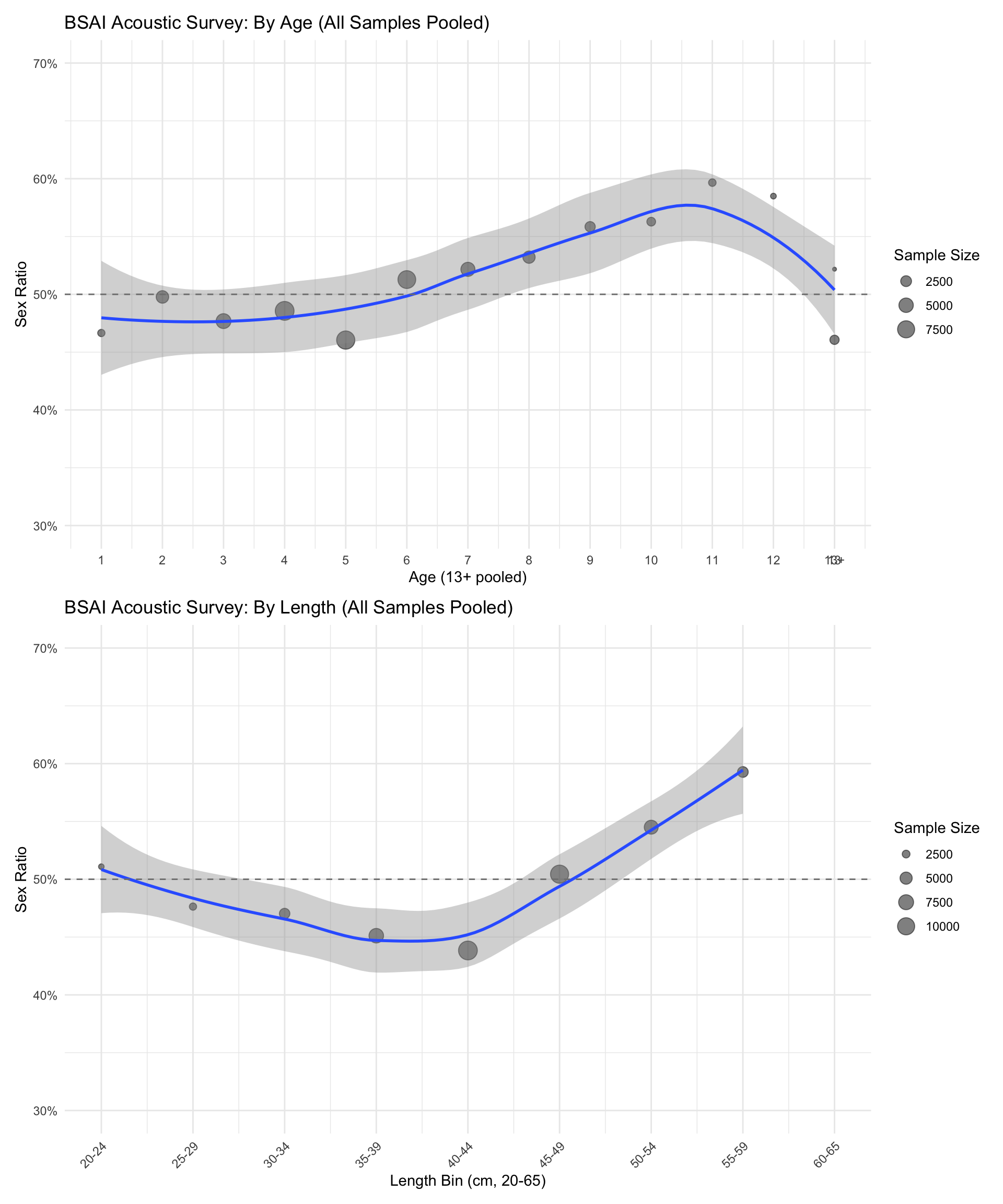
The all-years pooled Bering Sea summer acoustic-survey comparison is shown in Figure 11, with age-based sex ratios on the top panel and 5-cm length-bin sex ratios on the bottom panel.

Show code
p_age_overall <- df_acoust %>%
  filter(!is.na(AGE)) %>%
  plot_sex_ratio_age_box(min_n = 25, fmp_filter = "BSAI") +
  labs(title = "BSAI Acoustic Survey: By Age (All Samples Pooled)")

p_length_overall <- plot_sex_ratio_length_box(df_acoust, bin_width = 5, min_n = 25, fmp_filter = "BSAI") +
  labs(title = "BSAI Acoustic Survey: By Length (All Samples Pooled)")

p_age_overall / p_length_overall + patchwork::plot_layout(heights = c(1, 1))
Figure 11: BSAI pooled acoustic-survey sex ratios across all samples: by age with ages >13 pooled to 13+ (top) and by 5-cm length bins for lengths 20-65 cm (bottom).
2.2.1.2 By year

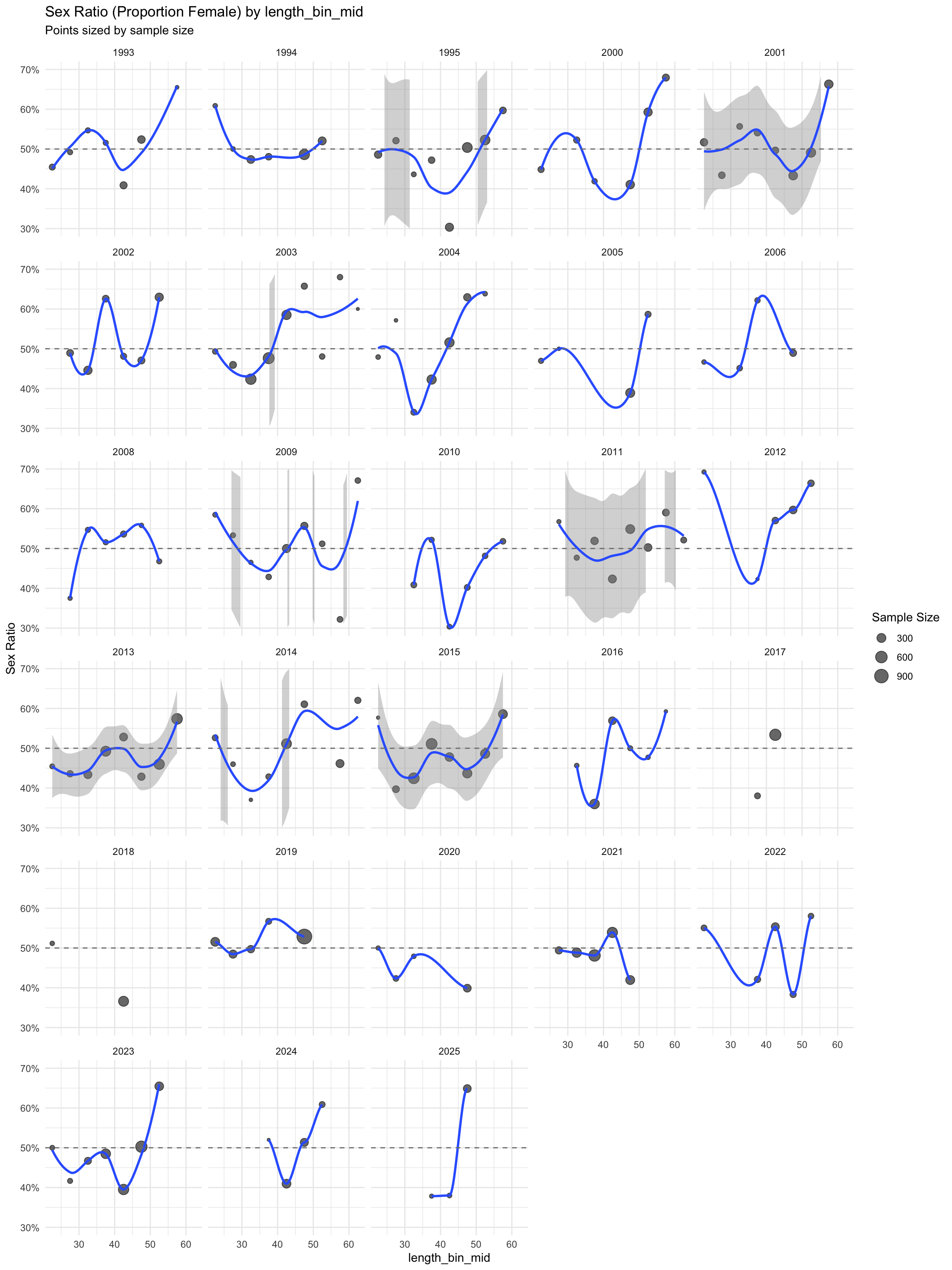
Year-specific Bering Sea summer acoustic-survey length-based sex ratios are shown in the annual-panel appendix (Figure 19).

2.2.2 GOA winter acoustic surveys

2.2.2.1 Aggregated over years

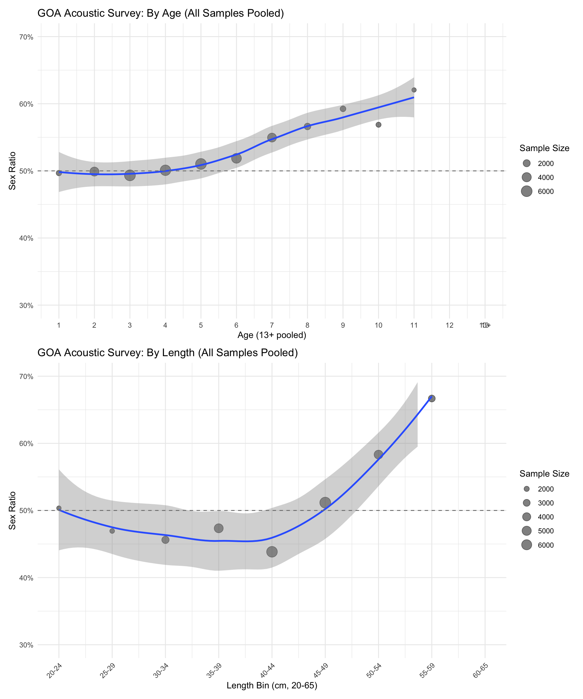
The all-years pooled GOA winter acoustic-survey comparison is shown in Figure 12, with age-based sex ratios on the top panel and 5-cm length-bin sex ratios on the bottom panel.

Show code
p_age_overall <- df_acoust %>%
  filter(!is.na(AGE)) %>%
  plot_sex_ratio_age_box(min_n = 25, fmp_filter = "GOA") +
  labs(title = "GOA Acoustic Survey: By Age (All Samples Pooled)")

p_length_overall <- plot_sex_ratio_length_box(df_acoust, bin_width = 5, min_n = 25, fmp_filter = "GOA") +
  labs(title = "GOA Acoustic Survey: By Length (All Samples Pooled)")

p_age_overall / p_length_overall + patchwork::plot_layout(heights = c(1, 1))
Figure 12: GOA pooled acoustic-survey sex ratios across all samples: by age with ages >13 pooled to 13+ (top) and by 5-cm length bins for lengths 20-65 cm (bottom).
2.2.2.2 By year

Year-specific GOA winter acoustic-survey length-based sex ratios are shown in the annual-panel appendix (Figure 20).

3 Methods (for evaluating fishery data)

To keep the Bayesian analysis tractable within a renderable Quarto workflow, the fitted models below use cell-aggregated data rather than all 1.4 million individual observations. The key design choice from the EDA is retained: fmp is treated as the primary split category, and separate models are fit for GOA and BSAI.

For sex ratio, the aggregated response is female count out of total F + M count within YEAR x season x subarea x age x 5-cm length-bin cells, excluding records coded U. Age 4 is used as the reference category so that the seasonB term is directly interpretable as the age-4 B-versus-A contrast after adjusting for length, year, and subarea. For growth, the aggregated response is mean length with its standard error within YEAR x season x subarea x sex x age cells, fit as a Gaussian measurement-error model. In both cases, the reduced formulation preserves the main contrasts of interest from the EDA: season, age, sex, year, subarea, and their comparison between GOA and BSAI.

The implemented brms data preparation was:

Show code
df_model <- df_age %>%
  filter(!is.na(SEX), !is.na(AGE), !is.na(LENGTH), !is.na(subarea))

sex_model_data <- df_model %>%
  filter(SEX %in% c("F", "M"), LENGTH >= 20, LENGTH <= 65) %>%
  mutate(
    female = if_else(SEX == "F", 1L, 0L),
    age_group = relevel(factor(pmin(as.integer(AGE), 13L)), ref = "4"),
    length_bin = pmin(floor((LENGTH - 20) / 5) * 5 + 20, 60),
    length_mid = if_else(length_bin == 60, 62.5, length_bin + 2.5)
  ) %>%
  group_by(fmp, YEAR, season, subarea, age_group, length_bin, length_mid) %>%
  summarise(female = sum(female), total_n = n(), .groups = "drop")

growth_model_data <- df_model %>%
  filter(SEX %in% c("F", "M"), AGE >= 2, AGE <= 10) %>%
  mutate(
    age_group = relevel(factor(as.integer(AGE)), ref = "4"),
    sex = relevel(factor(SEX), ref = "F")
  ) %>%
  group_by(fmp, YEAR, season, subarea, sex, age_group) %>%
  summarise(mean_length = mean(LENGTH), sd_length = sd(LENGTH), n = n(), .groups = "drop") %>%
  mutate(se_length = sd_length / sqrt(n)) %>%
  filter(is.finite(se_length), n >= 5)

The implemented brms model formulas were:

Show code
sex_formula <- bf(
  female | trials(total_n) ~ season * age_group + length_sc + year_sc + subarea
)

fit_sex_goa <- brm(
  sex_formula,
  data = filter(sex_model_data, fmp == "GOA"),
  family = binomial(),
  backend = "cmdstanr"
)

fit_sex_bsai <- brm(
  sex_formula,
  data = filter(sex_model_data, fmp == "BSAI"),
  family = binomial(),
  backend = "cmdstanr"
)
Show code
growth_formula <- bf(
  mean_length | se(se_length, sigma = TRUE) ~
    sex + season * age_group + sex:age_group + year_sc + subarea
)

fit_growth_goa <- brm(
  growth_formula,
  data = filter(growth_model_data, fmp == "GOA"),
  family = gaussian(),
  backend = "cmdstanr"
)

fit_growth_bsai <- brm(
  growth_formula,
  data = filter(growth_model_data, fmp == "BSAI"),
  family = gaussian(),
  backend = "cmdstanr"
)

4 Results

The reduced Bayesian fits support treating GOA and BSAI separately rather than pooling them into a single common model. Table Table 1 shows the aggregated datasets actually used in the fitted brms analyses.

Show code
model_data_summary %>%
  gt::gt() %>%
  gt::cols_label(
    outcome = "Outcome",
    fmp = "FMP",
    cells = "Aggregated Cells",
    source_n = "Fish Used",
    subareas = "Subareas"
  )
Table 1: Aggregated datasets used in the brms model fits.
Outcome FMP Aggregated Cells Fish Used Subareas
Sex ratio GOA 4456 64559 WGOA, CGOA
Sex ratio BSAI 5070 99116 SE_BS, NW_BS, AI
Growth GOA 1610 61678 WGOA, CGOA
Growth BSAI 1824 93725 SE_BS, NW_BS, AI

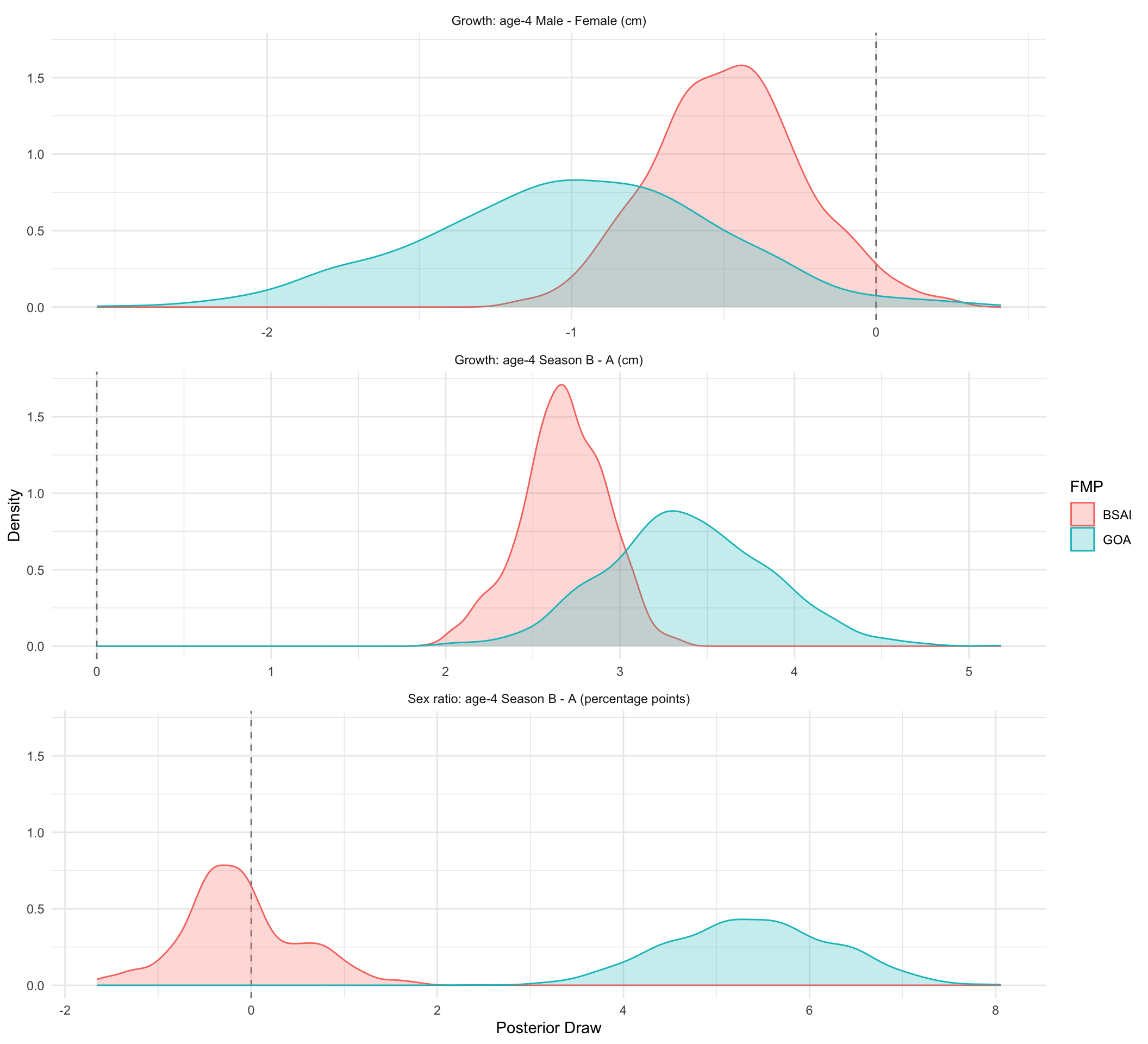
For sex ratio, the age-4 season contrast differs materially between GOA and BSAI. The posterior median B-versus-A change in female probability at age 4 was 5.4% in GOA (3.7% to 7.0%), but -0.2% in BSAI (-1.3% to 1.2%). That implies a clear positive seasonal shift in GOA sex ratio at age 4, whereas the comparable BSAI contrast overlaps zero.

For growth, the fitted models do not support the raw visual impression that age-4 fish are larger in Season A. After adjustment for age, sex, year, and subarea, the posterior median B-versus-A change in age-4 mean length was 3.36 cm in GOA (2.52 to 4.27 cm) and 2.68 cm in BSAI (2.17 to 3.12 cm). In both fmp groupings, the posterior age-4 seasonal effect is positive for Season B, which reverses the simple visual interpretation from the unadjusted EDA plots.

The fitted growth models also indicate that males are shorter than females at age 4 in both areas: -0.99 cm in GOA (-1.94 to -0.10 cm) and -0.48 cm in BSAI (-0.96 to 0.03 cm).

Table Table 2 summarizes the key posterior contrasts on interpretable scales, while Table Table 3 reports selected coefficient summaries from the separate GOA and BSAI fits. The sex-ratio coefficient table shows a positive season effect and stronger negative year trend in GOA, while both sex-ratio models estimate a positive length effect. The growth coefficient table shows positive Season B effects and negative male effects in both fmp groupings.

Show code
contrast_summary %>%
  select(contrast, fmp, estimate_display, cri_display) %>%
  gt::gt() %>%
  gt::cols_label(
    contrast = "Contrast",
    fmp = "FMP",
    estimate_display = "Posterior Median",
    cri_display = "95% CrI"
  )
Table 2: Key posterior contrasts from the separate GOA and BSAI brms fits.
Contrast FMP Posterior Median 95% CrI
Age-4 female probability: Season B - A GOA 5.4% 3.7% to 7.0%
Age-4 female probability: Season B - A BSAI -0.2% -1.3% to 1.2%
Age-4 mean length: Season B - A GOA 3.36 cm 2.52 to 4.27 cm
Age-4 mean length: Season B - A BSAI 2.68 cm 2.17 to 3.12 cm
Age-4 mean length: Male - Female GOA -0.99 cm -1.94 to -0.10 cm
Age-4 mean length: Male - Female BSAI -0.48 cm -0.96 to 0.03 cm
Show code
coefficient_summary %>%
  select(outcome, fmp, label, estimate_display, cri_display) %>%
  gt::gt(groupname_col = "outcome") %>%
  gt::cols_label(
    fmp = "FMP",
    label = "Parameter",
    estimate_display = "Posterior Median",
    cri_display = "95% CrI"
  )
Table 3: Selected coefficient summaries from the separate GOA and BSAI brms fits.
FMP Parameter Posterior Median 95% CrI
Sex ratio
GOA Season B effect at age 4 0.232 0.160 to 0.303
GOA Length effect (scaled) 0.700 0.666 to 0.730
GOA Year effect (scaled) -0.102 -0.117 to -0.086
BSAI Season B effect at age 4 -0.005 -0.056 to 0.052
BSAI Length effect (scaled) 0.907 0.886 to 0.929
BSAI Year effect (scaled) -0.018 -0.030 to -0.007
Growth
GOA Male effect at age 4 -1.000 -1.942 to -0.104
GOA Season B effect at age 4 3.383 2.522 to 4.268
GOA Year effect (scaled) 0.424 0.259 to 0.587
BSAI Male effect at age 4 -0.483 -0.964 to 0.029
BSAI Season B effect at age 4 2.675 2.165 to 3.122
BSAI Year effect (scaled) 0.260 0.171 to 0.349

The posterior marginal distributions in Figure 13 make the fmp differences more explicit. The season effect on sex ratio is clearly shifted positive in GOA and centered near zero in BSAI, whereas the growth contrasts are more similar between the two fmp groupings and remain positive for Season B in both cases.

Show code
ggplot(contrast_draws, aes(x = value, color = fmp, fill = fmp)) +
  geom_vline(xintercept = 0, linetype = "dashed", color = "gray50") +
  geom_density(alpha = 0.25) +
  facet_wrap(~contrast, scales = "free_x", ncol = 1) +
  labs(
    x = "Posterior Draw",
    y = "Density",
    color = "FMP",
    fill = "FMP"
  ) +
  theme_minimal(base_size = 11)
Figure 13: Posterior marginal distributions for key age-4 contrasts from separate GOA and BSAI brms models.

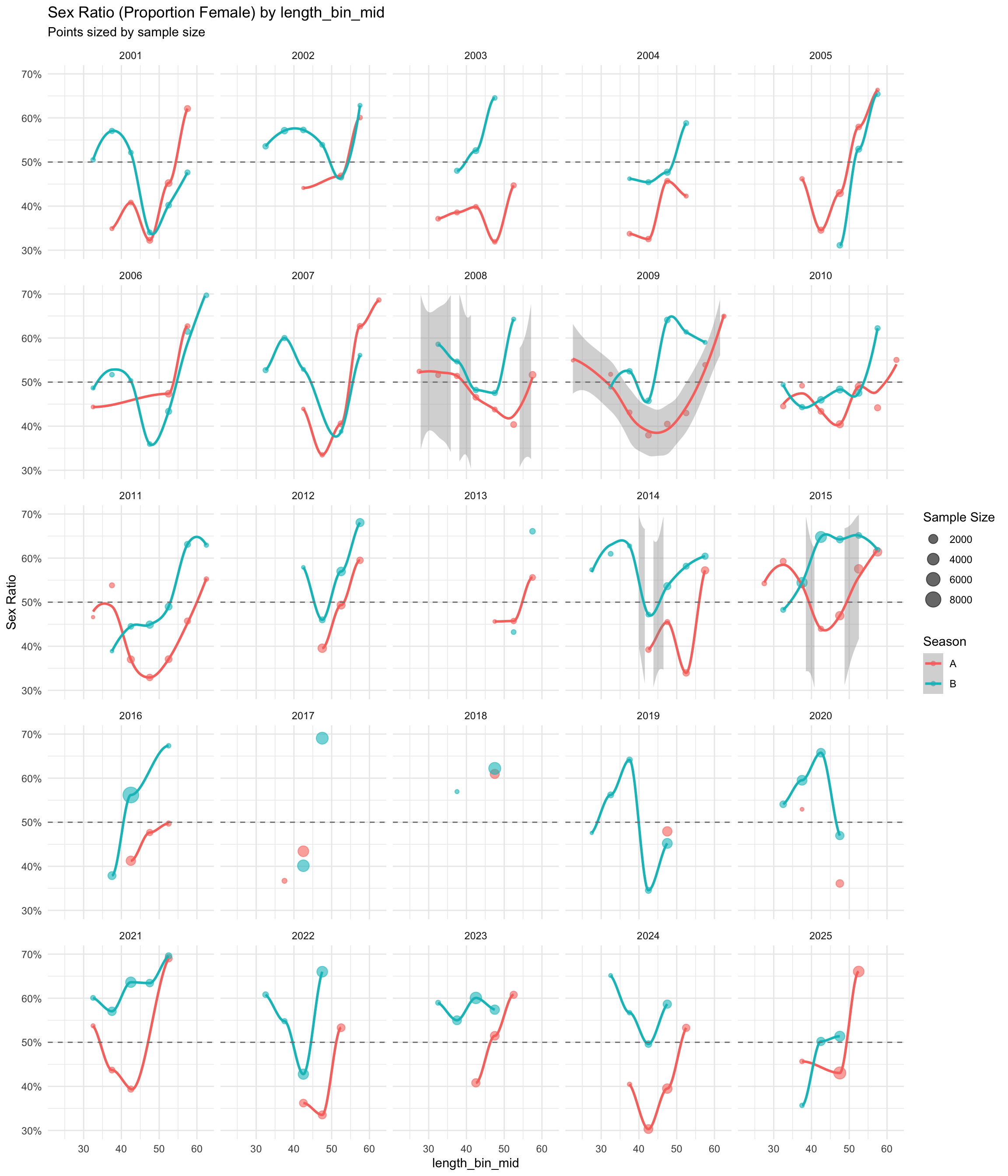
5 Appendix: Annual-panel figures

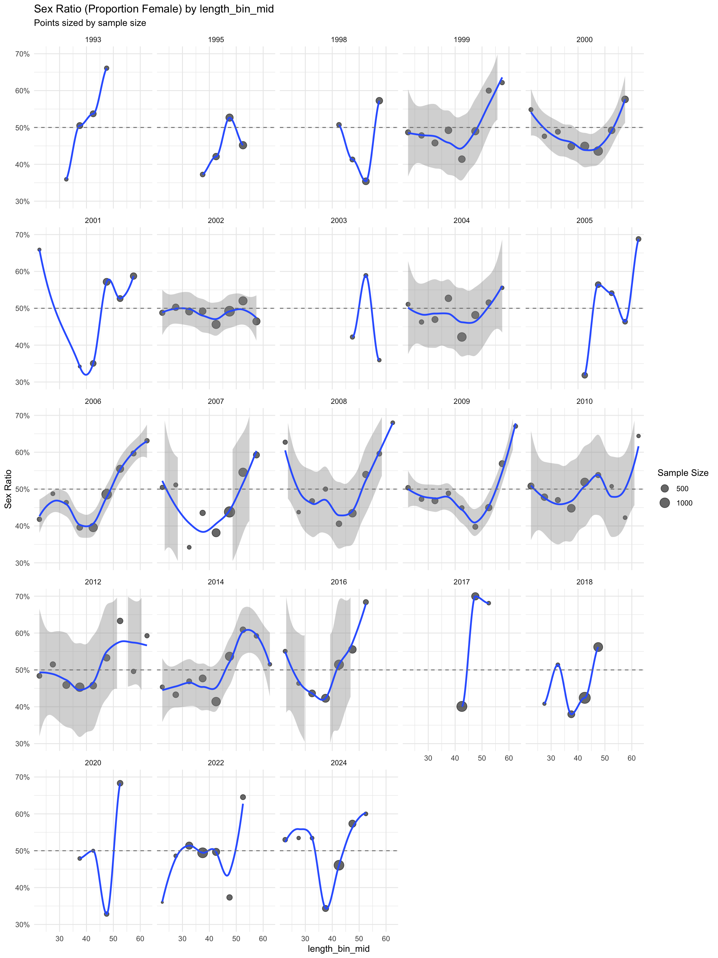
This appendix collects figures faceted by individual year. They remain linked from the exploratory narrative so the annual detail is available without interrupting the main sequence of pooled, seasonal, age, and spatial results.

5.1 Fishery annual panels

Show code
df_age_weekly |>
  filter(YEAR > 2000, between(week, 4, 14), total_n >= 25) |>
  ggplot(aes(x = week, y = sex_ratio)) +
  geom_hline(yintercept = 0.5, linetype = "dashed", color = "gray50") +
  geom_line(color = "#2C7FB8", linewidth = 0.5, alpha = 0.8) +
  geom_point(aes(size = total_n), color = "#2C7FB8", alpha = 0.7) +
  facet_wrap(vars(YEAR), ncol = 5) +
  scale_x_continuous(breaks = 4:14) +
  scale_y_continuous(labels = scales::percent, breaks = seq(0.3, 0.7, by = 0.1)) +
  scale_size_area(max_size = 5) +
  coord_cartesian(ylim = c(0.3, 0.7)) +
  labs(
    title = "BSAI CP A-season Sex Ratio by Week",
    subtitle = "CP records only; weeks 4-14; points sized by sample size",
    x = "ISO Calendar Week",
    y = "Sex Ratio",
    size = "Sample Size"
  ) +
  theme_minimal(base_size = 11)
Figure 14: BSAI catcher/processor (CP) A-season sex ratio (proportion female) by ISO calendar week and year for weeks 4-14. Only CP records are used. Points are sized by the number of female and male fish sampled; year-week cells with fewer than 25 fish are omitted.
Show code
df_age %>%
  filter(YEAR > 2000, LENGTH >= 20, LENGTH <= 65) %>%
  mutate(length_bin_mid = if_else(
    pmin(floor((LENGTH - 20) / 5) * 5 + 20, 60) == 60,
    62.5,
    pmin(floor((LENGTH - 20) / 5) * 5 + 20, 60) + 2.5
  )) %>%
  plot_sex_ratio(
    x_var = length_bin_mid,
    facet_var = YEAR,
    min_n = 100,
    show_labels = FALSE,
    facet_ncol = 5,
    fmp_filter = "GOA",
    color_var = "season"
  )
Figure 15: Sex ratio (proportion female) by 5-cm length bins for GOA, faceted by year with season shown by color (YEAR > 2000; min_n = 100).
Show code
df_age %>%
  filter(YEAR > 2000) %>%
  plot_sex_ratio(
    x_var = LENGTH,
    facet_var = YEAR,
    min_n = 500,
    show_labels = FALSE,
    facet_ncol = 5,
    fmp_filter = "BSAI"
  )
Figure 16: Sex ratio (proportion female) by length for BSAI, faceted by year (YEAR > 2000; min_n = 500).
Show code
df_age %>%
  filter(YEAR > 2000) %>%
  plot_sex_ratio(
    x_var = AGE,
    facet_var = YEAR,
    show_labels = FALSE,
    facet_ncol = 5,
    fmp_filter = "GOA"
  )
Figure 17: Sex ratio (proportion female) by age for GOA, faceted by year (YEAR > 2000).
Show code
df_age %>%
  filter(YEAR > 2000) %>%
  plot_sex_ratio(
    x_var = AGE,
    facet_var = YEAR,
    show_labels = FALSE,
    facet_ncol = 5,
    fmp_filter = "BSAI"
  )
Figure 18: Sex ratio (proportion female) by age for BSAI, faceted by year (YEAR > 2000).

5.2 Acoustic-survey annual panels

Show code
df_acoust %>%
  filter(LENGTH >= 20, LENGTH <= 65) %>%
  mutate(length_bin_mid = if_else(
    pmin(floor((LENGTH - 20) / 5) * 5 + 20, 60) == 60,
    62.5,
    pmin(floor((LENGTH - 20) / 5) * 5 + 20, 60) + 2.5
  )) %>%
  plot_sex_ratio(
    x_var = length_bin_mid,
    facet_var = YEAR,
    min_n = 25,
    show_labels = FALSE,
    facet_ncol = 5,
    fmp_filter = "BSAI"
  )
Figure 19: Acoustic survey sex ratio (proportion female) by 5-cm length bins for BSAI, faceted by year (1993-2024; min_n = 25).
Show code
df_acoust %>%
  filter(LENGTH >= 20, LENGTH <= 65) %>%
  mutate(length_bin_mid = if_else(
    pmin(floor((LENGTH - 20) / 5) * 5 + 20, 60) == 60,
    62.5,
    pmin(floor((LENGTH - 20) / 5) * 5 + 20, 60) + 2.5
  )) %>%
  plot_sex_ratio(
    x_var = length_bin_mid,
    facet_var = YEAR,
    min_n = 25,
    show_labels = FALSE,
    facet_ncol = 5,
    fmp_filter = "GOA"
  )
Figure 20: Acoustic survey sex ratio (proportion female) by 5-cm length bins for GOA, faceted by year (1993-2025; min_n = 25).

6 References

  • Source script: otoliths.R (BSAI pollock fisheries otolith selector; created 2021-03-02).
  • Input data used here: df_age.csv (derived analysis dataset with public-safe columns only).
  • Query workflow used to generate age data is documented in GetAgesSql.R.
  • Ianelli, J., T. Honkalehto, S. Wassermann, A. McCarthy, S. Steinessen, C. McGilliard, and E. Siddon. 2024. Assessment of walleye pollock in the eastern Bering Sea. North Pacific Fishery Management Council, Anchorage, AK.