filter_plot_data <- function(data, season_filter = NULL, fmp_filter = NULL) {
data <- data %>%
filter(SEX %in% c("F", "M"))
if (!is.null(season_filter)) {
data <- data %>%
filter(season %in% season_filter)
}
if (!is.null(fmp_filter)) {
data <- data %>%
filter(fmp %in% fmp_filter)
}
data
}
summarize_sex_ratio <- function(data, group_vars) {
data %>%
group_by(!!!group_vars) %>%
summarize(
female_n = sum(SEX == "F"),
male_n = sum(SEX == "M"),
total_n = female_n + male_n,
sex_ratio = female_n / total_n,
.groups = "drop"
)
}
build_facet_vars <- function(primary_facet = NULL, facet_season = FALSE, facet_fmp = FALSE) {
facet_vars <- list()
if (!is.null(primary_facet) && !rlang::quo_is_null(primary_facet)) {
facet_vars <- c(facet_vars, list(primary_facet))
}
if (facet_season) {
facet_vars <- c(facet_vars, rlang::quos(season))
}
if (facet_fmp) {
facet_vars <- c(facet_vars, rlang::quos(fmp))
}
facet_vars
}
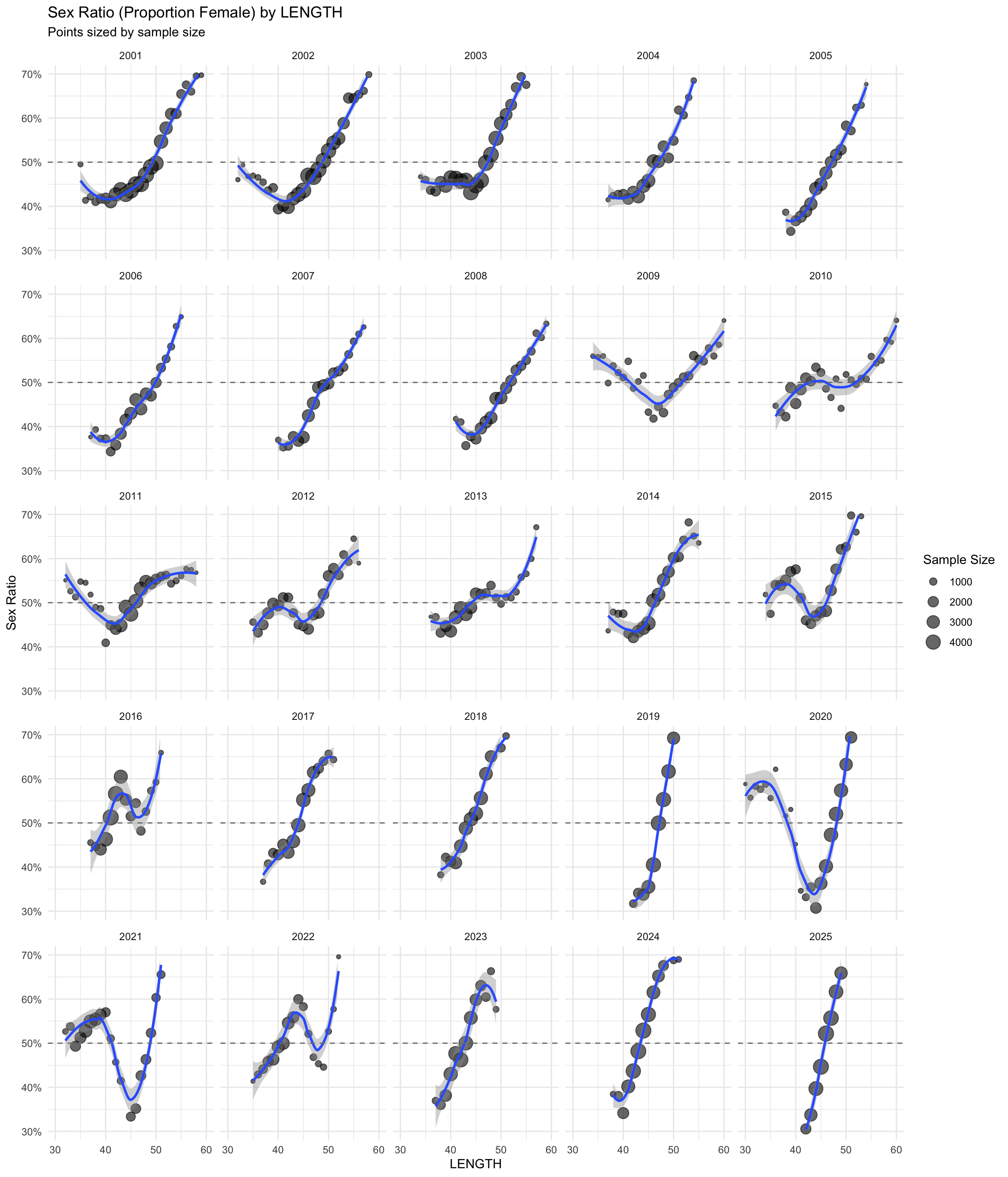
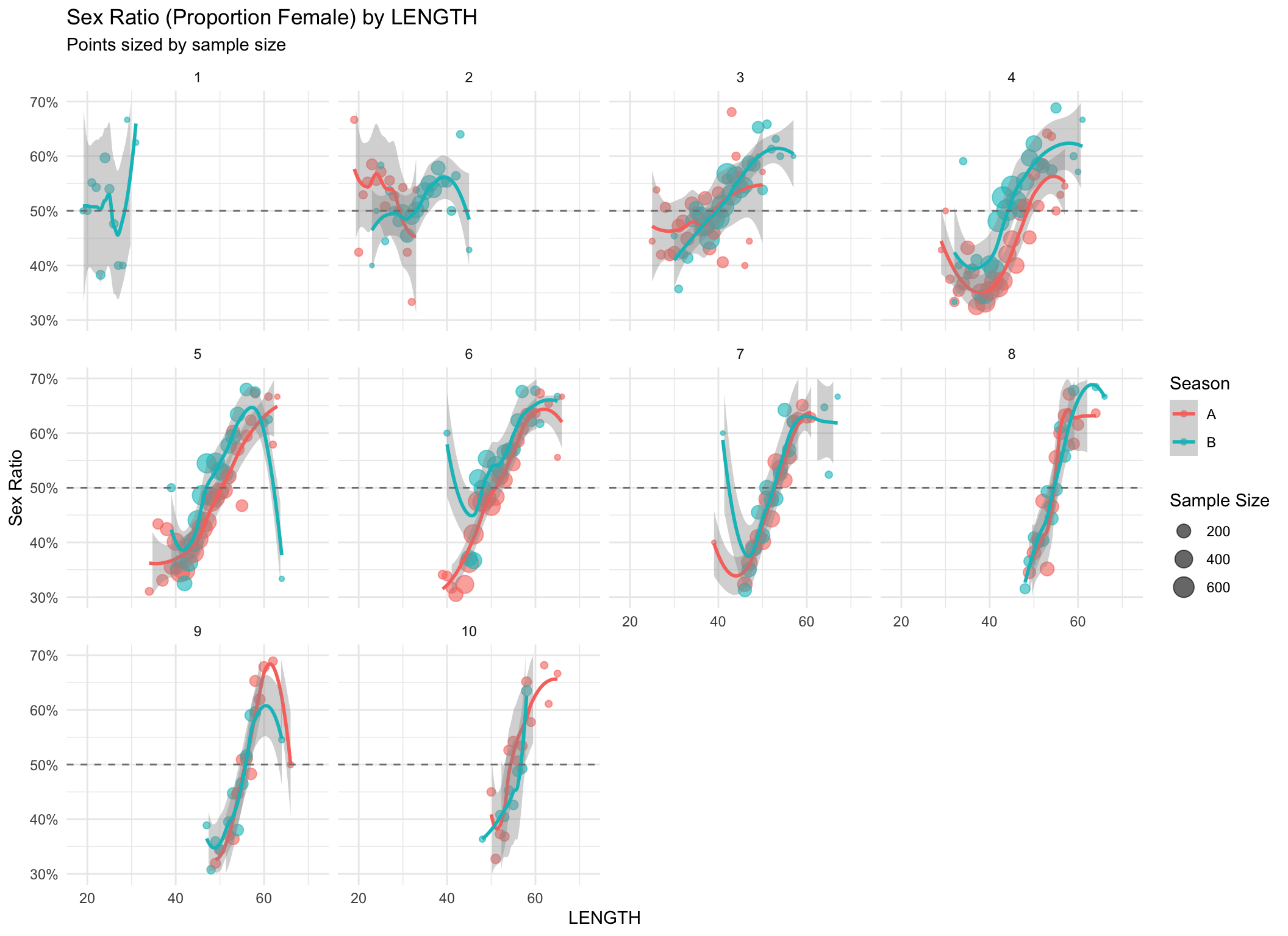
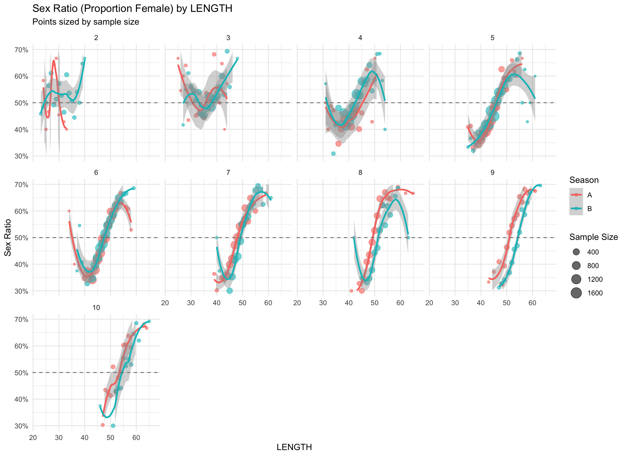
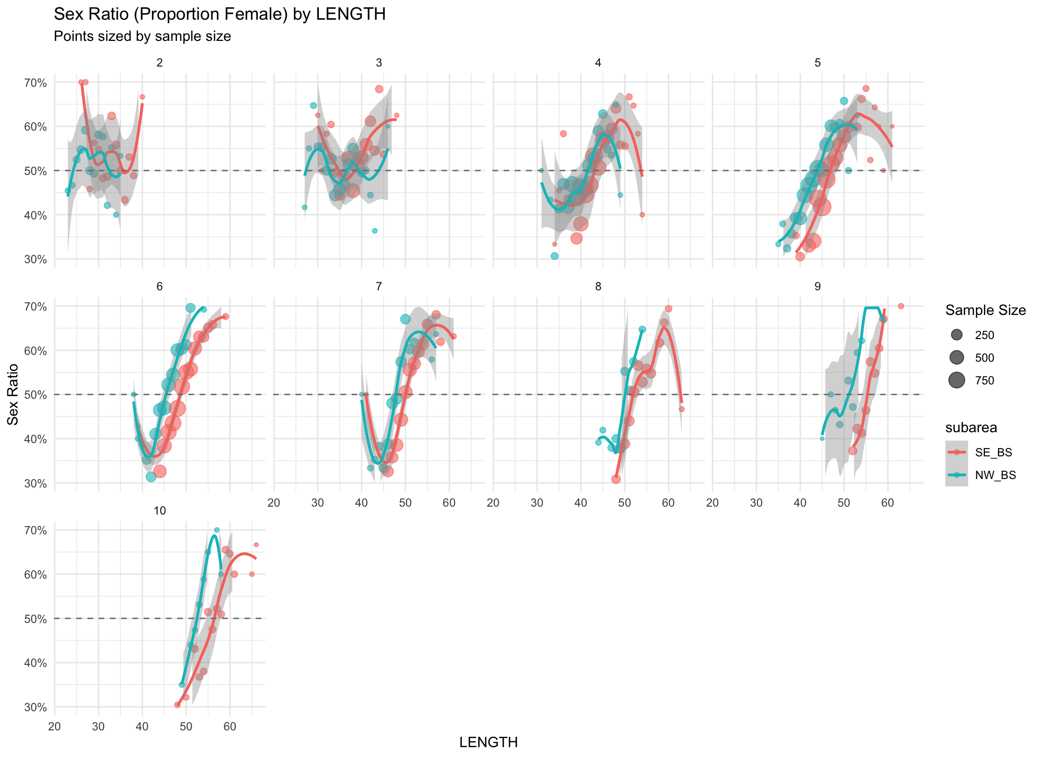
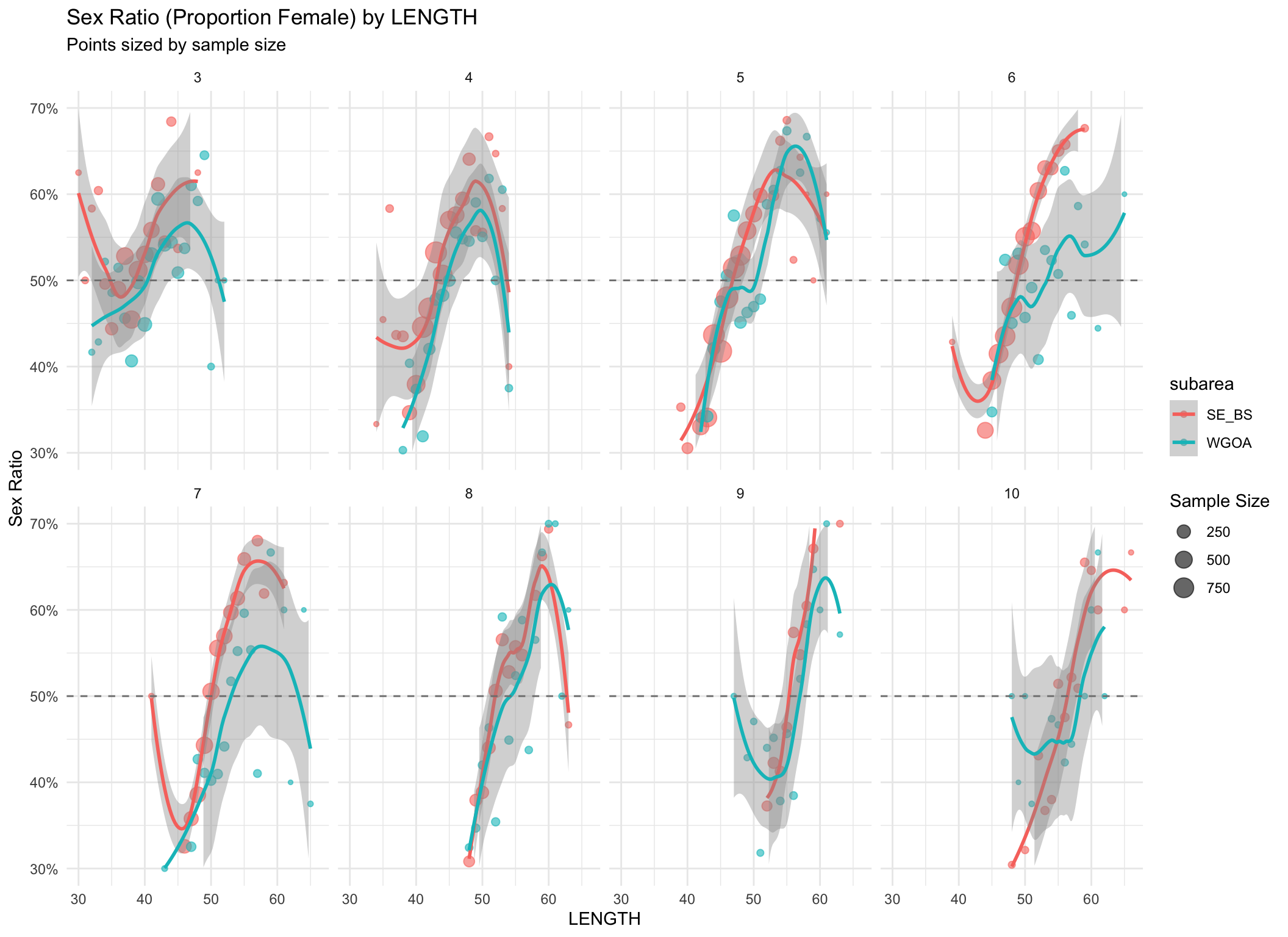
plot_sex_ratio <- function(data, x_var, facet_var = NULL, min_n = 5,
y_limits = c(0.3, 0.7), show_labels = FALSE,
facet_ncol = 6, season_filter = NULL,
fmp_filter = NULL, facet_season = FALSE,
facet_fmp = FALSE, color_var = NULL) {
x_var <- rlang::enquo(x_var)
facet_var <- rlang::enquo(facet_var)
facet_vars <- build_facet_vars(facet_var, facet_season = facet_season, facet_fmp = facet_fmp)
color_sym <- if (is.null(color_var)) NULL else rlang::sym(color_var)
group_vars <- c(facet_vars, list(x_var), if (is.null(color_sym)) list() else list(color_sym))
plot_df <- data %>%
filter_plot_data(season_filter = season_filter, fmp_filter = fmp_filter) %>%
summarize_sex_ratio(group_vars) %>%
filter(total_n >= min_n)
plot_mapping <- aes(x = !!x_var, y = sex_ratio)
if (!is.null(color_sym)) {
plot_mapping$colour <- color_sym
}
color_label <- if (is.null(color_var)) {
NULL
} else {
dplyr::case_match(
color_var,
"season" ~ "Season",
"fmp" ~ "FMP",
.default = color_var
)
}
p <- ggplot(plot_df, plot_mapping)
if (show_labels) {
p <- p +
geom_text(
aes(label = round(total_n / 100, 1)),
size = 2.8,
alpha = 0.8,
check_overlap = TRUE
)
} else {
p <- p +
geom_point(aes(size = total_n), alpha = 0.6)
}
p <- p +
geom_smooth(method = "loess", formula = "y ~ x") +
geom_hline(yintercept = 0.5, linetype = "dashed", color = "gray50") +
scale_y_continuous(labels = scales::percent, limits = y_limits) +
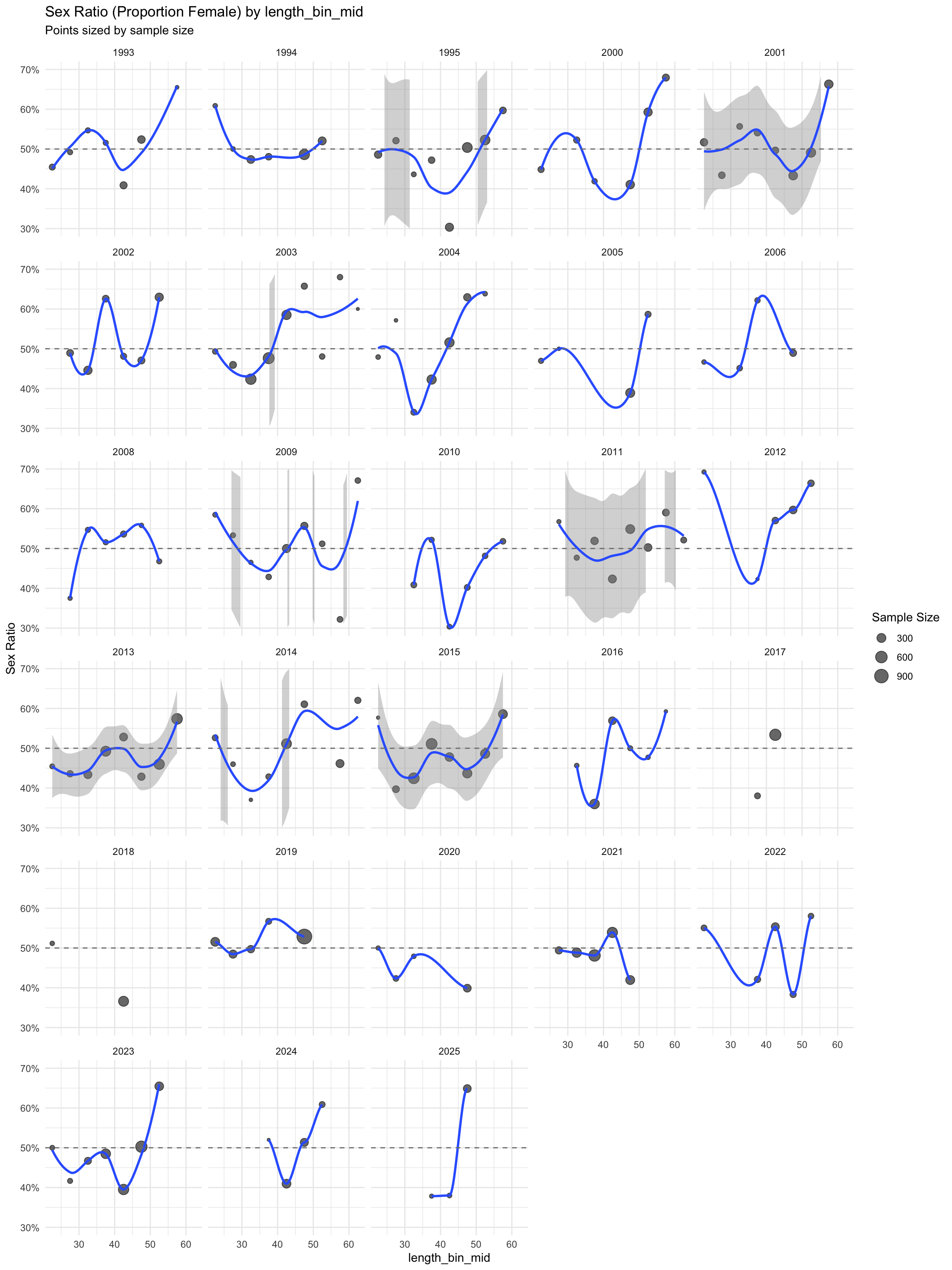
labs(
title = paste("Sex Ratio (Proportion Female) by", rlang::as_label(x_var)),
subtitle = if (show_labels) "Labels show Sample Size / 100" else "Points sized by sample size",
x = rlang::as_label(x_var),
y = "Sex Ratio",
size = "Sample Size",
color = color_label
) +
theme_minimal(base_size = 11)
if (length(facet_vars) > 0) {
p <- p + facet_wrap(vars(!!!facet_vars), ncol = facet_ncol)
}
p
}
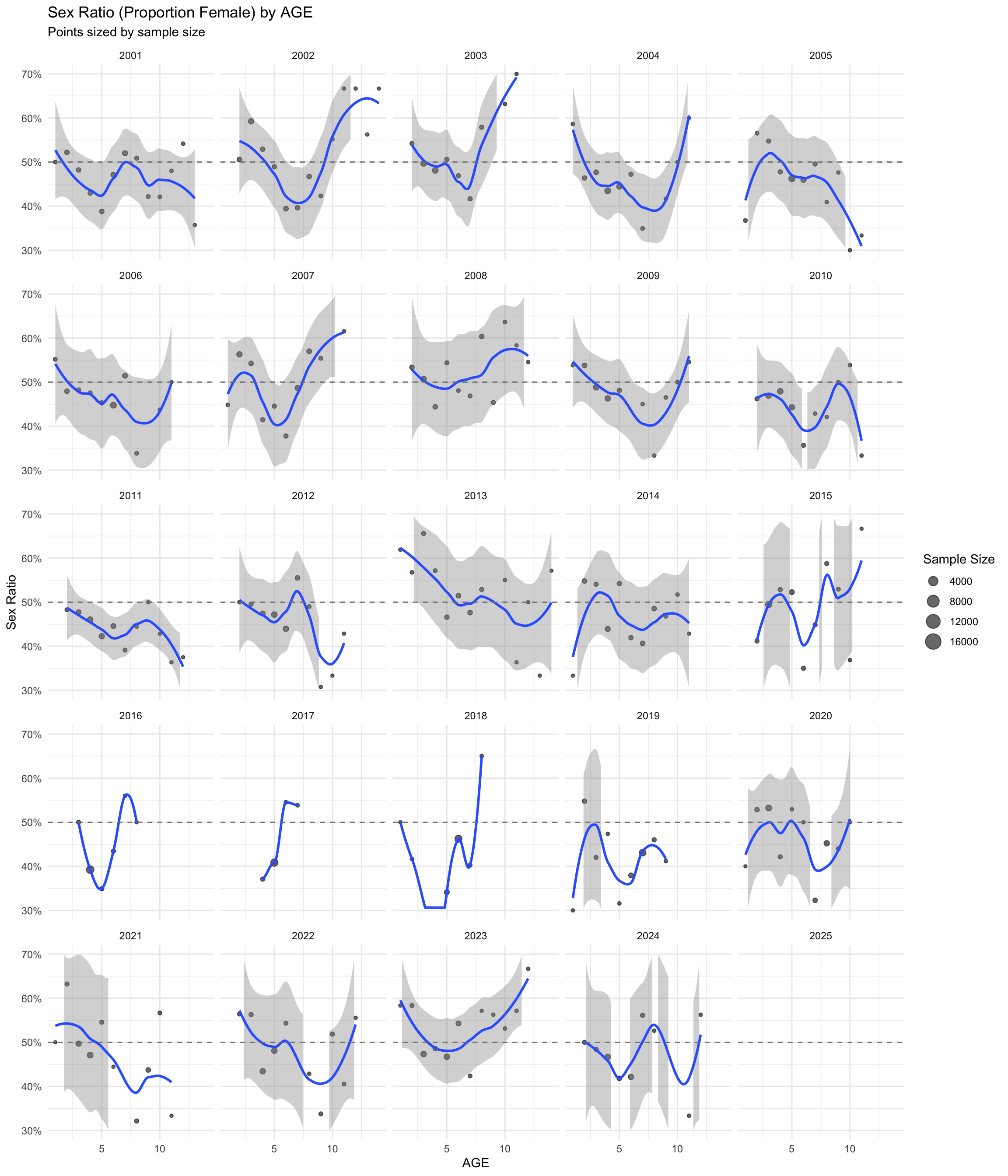
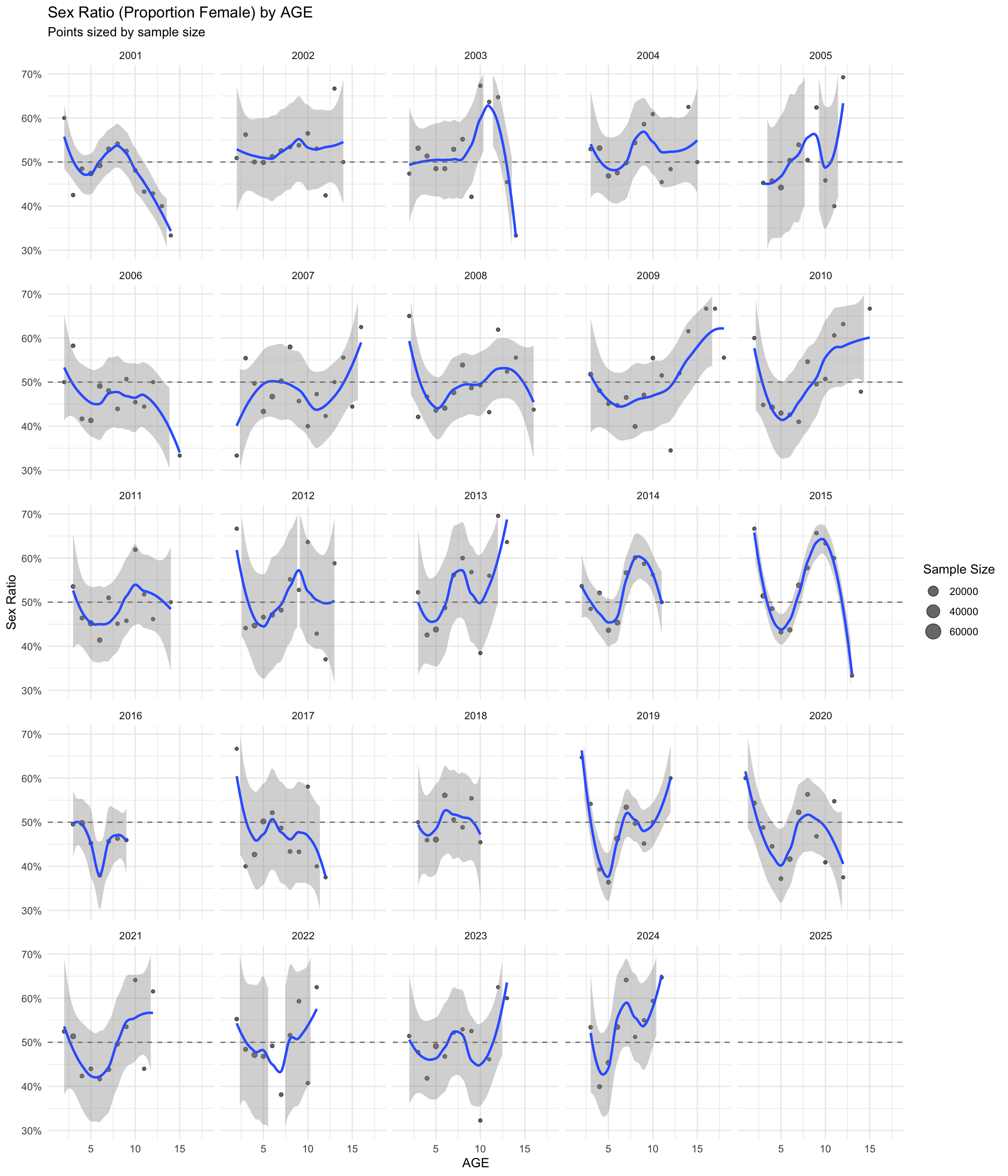
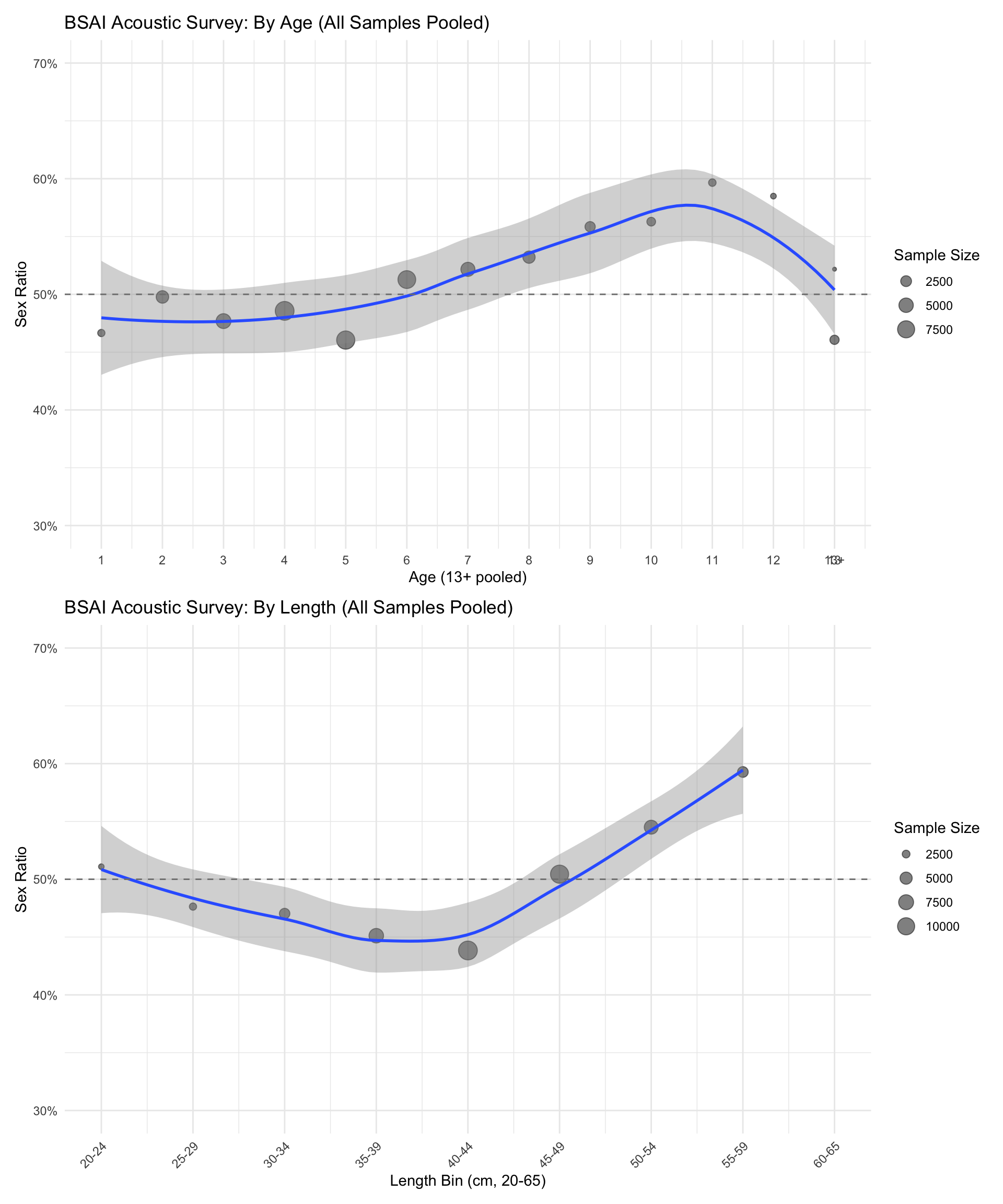
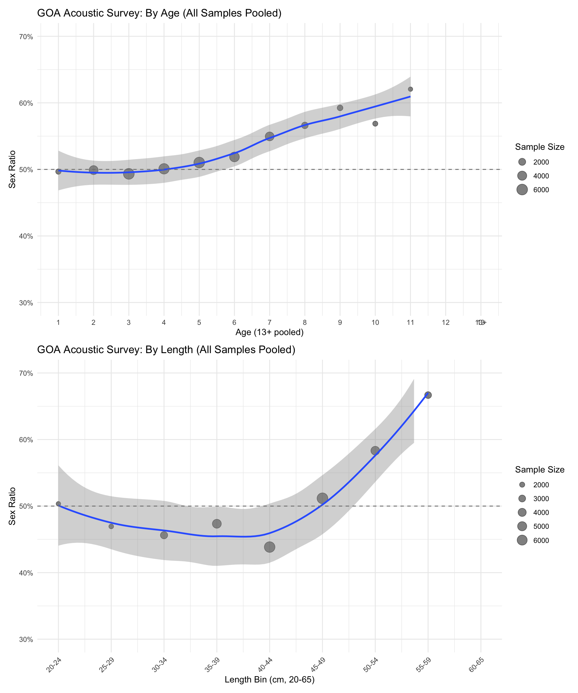
plot_sex_ratio_age_box <- function(data, min_n = 25, y_limits = c(0.3, 0.7),
facet_ncol = 6, season_filter = NULL,
fmp_filter = NULL, facet_season = FALSE,
facet_fmp = FALSE) {
facet_vars <- build_facet_vars(facet_season = facet_season, facet_fmp = facet_fmp)
group_vars <- c(facet_vars, rlang::quos(age_group))
plot_df <- data %>%
filter_plot_data(season_filter = season_filter, fmp_filter = fmp_filter) %>%
mutate(
age_group = if_else(AGE > 13, "13+", as.character(AGE))
) %>%
summarize_sex_ratio(group_vars) %>%
filter(total_n >= min_n)
numeric_ages <- suppressWarnings(as.integer(plot_df$age_group[plot_df$age_group != "13+"]))
age_levels <- c(
as.character(sort(unique(numeric_ages[!is.na(numeric_ages)]))),
if (any(plot_df$age_group == "13+")) "13+" else character(0)
)
plot_df <- plot_df %>%
mutate(
age_group = factor(age_group, levels = age_levels),
age_num = if_else(age_group == "13+", 13, as.numeric(as.character(age_group)))
)
p <- ggplot(plot_df, aes(x = age_num, y = sex_ratio)) +
geom_point(aes(size = total_n), alpha = 0.5) +
geom_smooth(method = "loess", formula = "y ~ x") +
geom_hline(yintercept = 0.5, linetype = "dashed", color = "gray50") +
scale_y_continuous(labels = scales::percent, limits = y_limits) +
scale_x_continuous(
breaks = c(as.integer(age_levels[age_levels != "13+"]), if ("13+" %in% age_levels) 13 else numeric(0)),
labels = age_levels
) +
labs(
x = "Age (13+ pooled)",
y = "Sex Ratio",
size = "Sample Size"
) +
theme_minimal(base_size = 11)
if (length(facet_vars) > 0) {
p <- p + facet_wrap(vars(!!!facet_vars), ncol = facet_ncol)
}
p
}
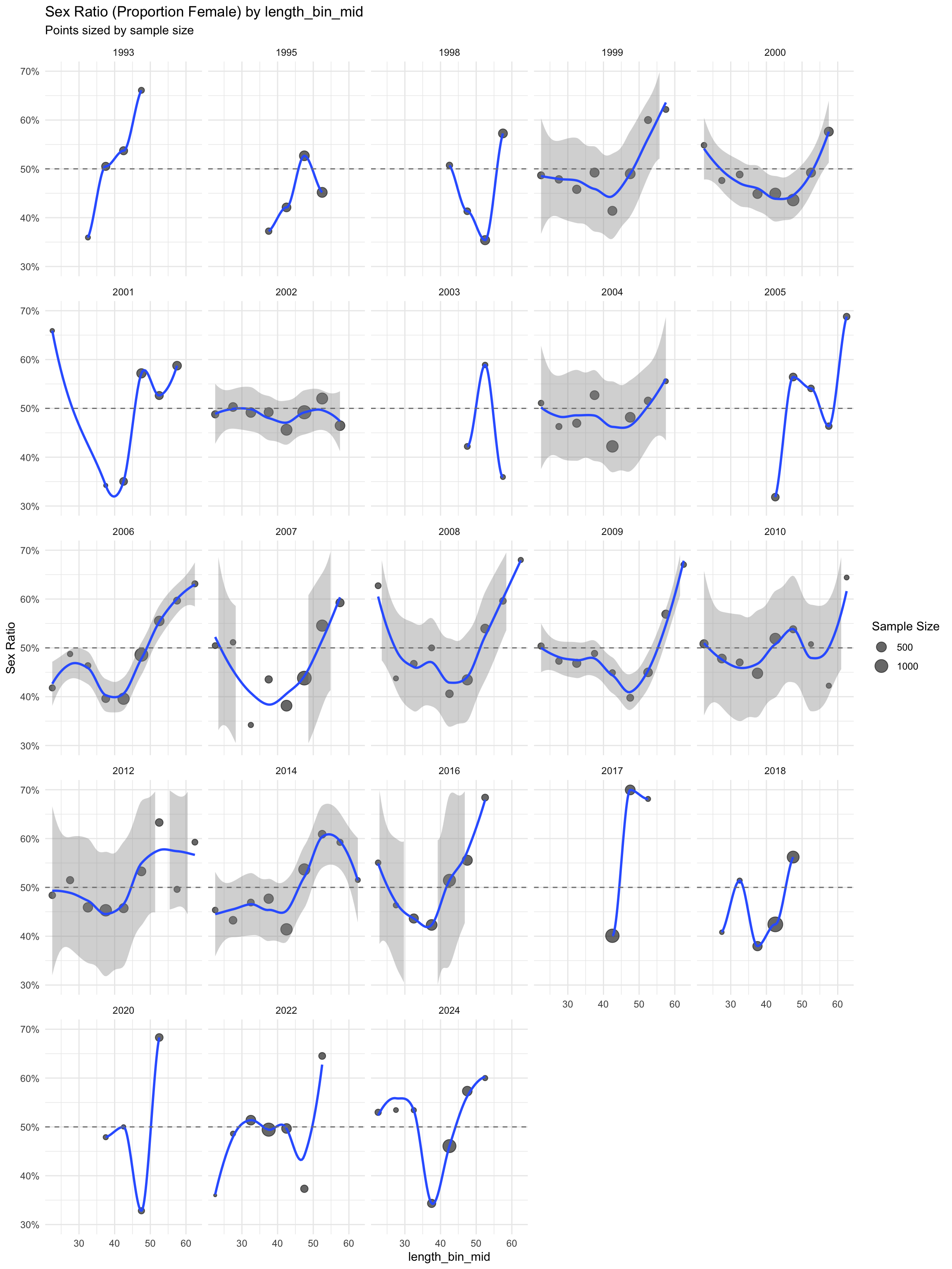
plot_sex_ratio_length_box <- function(data, bin_width = 5, min_n = 50,
y_limits = c(0.3, 0.7), facet_ncol = 6,
season_filter = NULL, fmp_filter = NULL,
facet_season = FALSE, facet_fmp = FALSE) {
facet_vars <- build_facet_vars(facet_season = facet_season, facet_fmp = facet_fmp)
group_vars <- c(facet_vars, rlang::quos(length_bin_lower))
plot_df <- data %>%
filter_plot_data(season_filter = season_filter, fmp_filter = fmp_filter) %>%
filter(LENGTH >= 20, LENGTH <= 65) %>%
mutate(
length_bin_lower = pmin(floor((LENGTH - 20) / bin_width) * bin_width + 20, 60)
) %>%
summarize_sex_ratio(group_vars) %>%
filter(total_n >= min_n) %>%
mutate(
length_bin_mid = if_else(length_bin_lower == 60, 62.5, length_bin_lower + bin_width / 2),
length_bin = if_else(
length_bin_lower == 60,
"60-65",
paste0(length_bin_lower, "-", length_bin_lower + (bin_width - 1))
),
length_bin = factor(length_bin, levels = unique(length_bin[order(length_bin_lower)]))
)
p <- ggplot(plot_df, aes(x = length_bin_mid, y = sex_ratio)) +
geom_point(aes(size = total_n), alpha = 0.5) +
geom_smooth(method = "loess", formula = "y ~ x") +
geom_hline(yintercept = 0.5, linetype = "dashed", color = "gray50") +
scale_y_continuous(labels = scales::percent, limits = y_limits) +
scale_x_continuous(
breaks = unique(plot_df$length_bin_mid[order(plot_df$length_bin_lower)]),
labels = unique(plot_df$length_bin[order(plot_df$length_bin_lower)])
) +
labs(
x = "Length Bin (cm, 20-65)",
y = "Sex Ratio",
size = "Sample Size"
) +
theme_minimal(base_size = 11) +
theme(axis.text.x = element_text(angle = 45, hjust = 1))
if (length(facet_vars) > 0) {
p <- p + facet_wrap(vars(!!!facet_vars), ncol = facet_ncol)
}
p
}
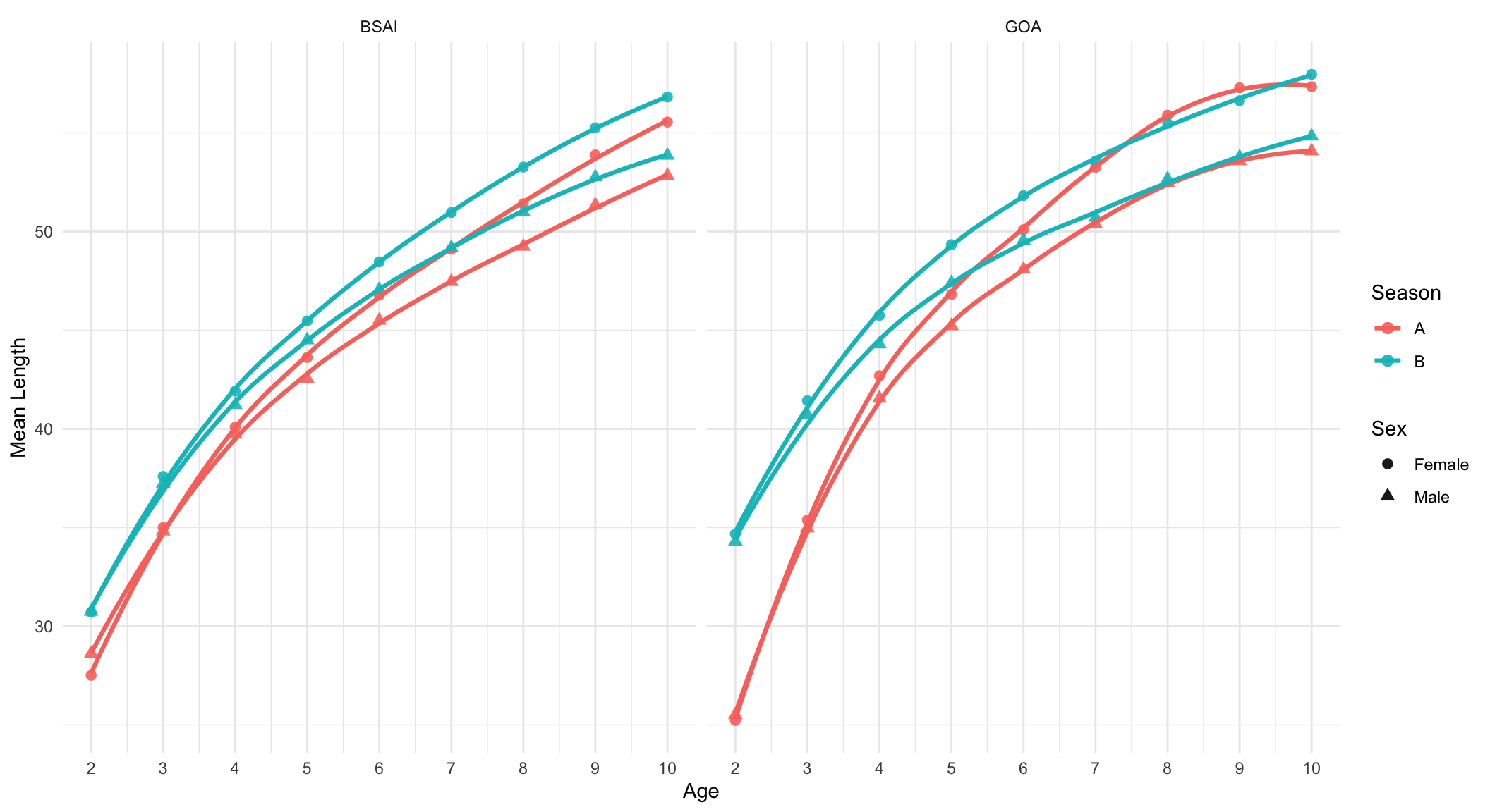
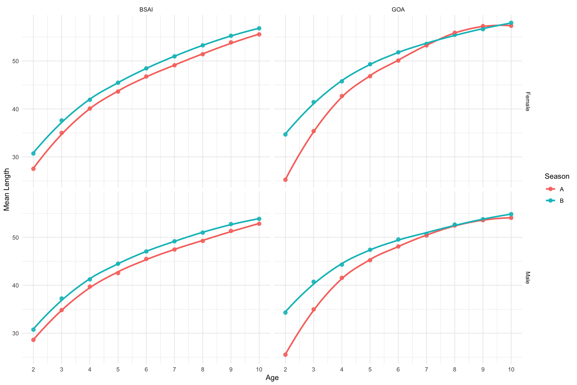
plot_mean_length_age_sex <- function(data, age_range = 2:10, facet_ncol = 6,
season_filter = NULL, fmp_filter = NULL,
facet_season = FALSE, facet_fmp = FALSE,
facet_sex = FALSE, color_var = "sex",
shape_var = NULL, facet_rows = NULL,
facet_cols = NULL, linetype_var = NULL) {
facet_names <- c(
if (facet_season) "season",
if (facet_fmp) "fmp",
if (facet_sex) "sex"
)
facet_grid_names <- c(facet_rows, facet_cols)
group_names <- unique(c(facet_names, facet_grid_names, "age_num", "sex", color_var, shape_var, linetype_var))
plot_df <- data %>%
filter_plot_data(season_filter = season_filter, fmp_filter = fmp_filter) %>%
filter(!is.na(AGE), !is.na(LENGTH)) %>%
mutate(
age_num = as.numeric(AGE),
sex = recode(SEX, F = "Female", M = "Male")
) %>%
filter(age_num >= min(age_range), age_num <= max(age_range)) %>%
group_by(across(all_of(group_names))) %>%
summarize(
mean_length = mean(LENGTH, na.rm = TRUE),
.groups = "drop"
)
plot_mapping <- aes(x = age_num, y = mean_length)
plot_mapping$colour <- rlang::sym(color_var)
if (!is.null(shape_var)) {
plot_mapping$shape <- rlang::sym(shape_var)
}
if (!is.null(linetype_var)) {
plot_mapping$linetype <- rlang::sym(linetype_var)
}
line_group_names <- unique(c(color_var, shape_var, linetype_var, if (!facet_sex) "sex"))
plot_mapping$group <- rlang::expr(interaction(!!!rlang::syms(line_group_names), drop = TRUE))
color_label <- dplyr::case_match(
color_var,
"sex" ~ "Sex",
"season" ~ "Season",
"fmp" ~ "FMP",
.default = color_var
)
shape_label <- if (is.null(shape_var)) {
NULL
} else {
dplyr::case_match(
shape_var,
"sex" ~ "Sex",
"season" ~ "Season",
"fmp" ~ "FMP",
.default = shape_var
)
}
linetype_label <- if (is.null(linetype_var)) {
NULL
} else {
dplyr::case_match(
linetype_var,
"sex" ~ "Sex",
"season" ~ "Season",
"fmp" ~ "FMP",
.default = linetype_var
)
}
p <- ggplot(plot_df, plot_mapping) +
geom_point(size = 2.4, alpha = 0.9) +
geom_smooth(method = "loess", formula = "y ~ x", se = FALSE, linewidth = 1.1) +
scale_x_continuous(breaks = age_range) +
labs(
x = "Age",
y = "Mean Length",
color = color_label,
shape = shape_label,
linetype = linetype_label
) +
theme_minimal(base_size = 11)
if (!is.null(facet_rows) || !is.null(facet_cols)) {
row_vars <- if (is.null(facet_rows)) list(.) else rlang::syms(facet_rows)
col_vars <- if (is.null(facet_cols)) list(.) else rlang::syms(facet_cols)
p <- p + facet_grid(rows = vars(!!!row_vars), cols = vars(!!!col_vars))
} else if (length(facet_names) > 0) {
p <- p + facet_wrap(vars(!!!rlang::syms(facet_names)), ncol = facet_ncol)
}
p
}